Posted on

Lane markers detection

Michal Polko

In this project, we detect lane markers in videos taken with dashboard camera.

Process

  1. Convert a video frame to grayscale, boost contrast and apply dilation operator to highlight lane markers in the frame.
    polko_highlighted_markers
    Highlighted lane markers.
    cvtColor(frame, frame_bw, CV_RGB2GRAY);
    frame_bw.convertTo(frame_bw, CV_32F, 1.0 / 255.0);
    pow(frame_bw, 3.0, frame_bw);
    frame_bw *= 3.0;
    frame_bw.convertTo(frame_bw, CV_8U, 255.0);
    dilate(frame_bw, frame_bw, getStructuringElement(CV_SHAPE_RECT, Size(3, 3)));
    
  2. Apply the Canny edge detection to find edges.
    polko_edges
    Application of the Canny edge detection.
    int cny_threshold = 100;
    Canny(frame_bw, frame_edges, cny_threshold, cny_threshold * 3, 3);
    
  3. Apply the Hough transform to find line segments.
    vector<Vec4i> hg_lines;
    HoughLinesP(frame_edges, hg_lines, 1, CV_PI / 180, 15, 15, 2);
    
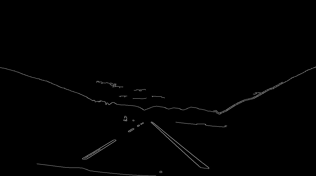
  4. Since the Hough transform returns all line segments, not only those around lane markers, it is necessary to filter the results.
    1. We create two lines that describe boundaries of the current lane (hypothesis).
      1. We place two converging lines in the frame.
      2. Using brute-force search, we try to find position where they capture as many line segments as possible.
      3. Since road in the frame can have more than one lane, we try to find result as narrow as possible.
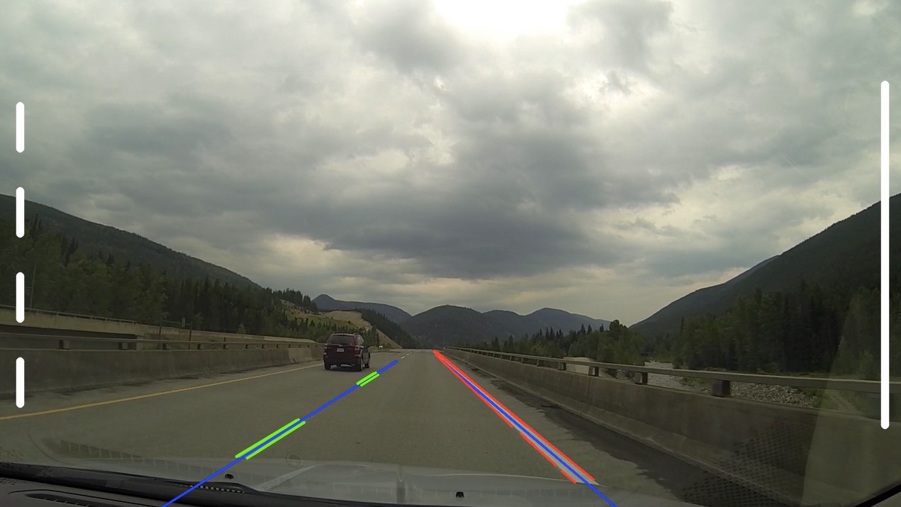
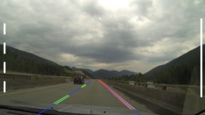
    2. We select line segments that are captured by the created hypothesis, mark them as lane markers and draw them.
    3. Each frame, we take the detected lane markers from the previous frame and perform linear regression to adjust the hypothesis (continuous adjustment).
    4. If we cannot find lane markers in more than 5 successive frames (due to failure of continuous adjustment, lane change, intersection, …), we create a new hypothesis.
    5. If the hypothesis is too wide (almost full width of the frame), we create a new one, because arrangement of road lanes might have changed (e.g. additional lane on freeway).
  5. To distinguish between solid and dashed lane markers, we calculate coverage of the hypothesis by line segments. If the coverage is less than 60%, it is a dashed line; if more, it is a solid line.

    polko_result
    Filtered result of the Hough transform + detection of solid/dashed lines.
Posted on

Free parking spots detection

Jan Onder

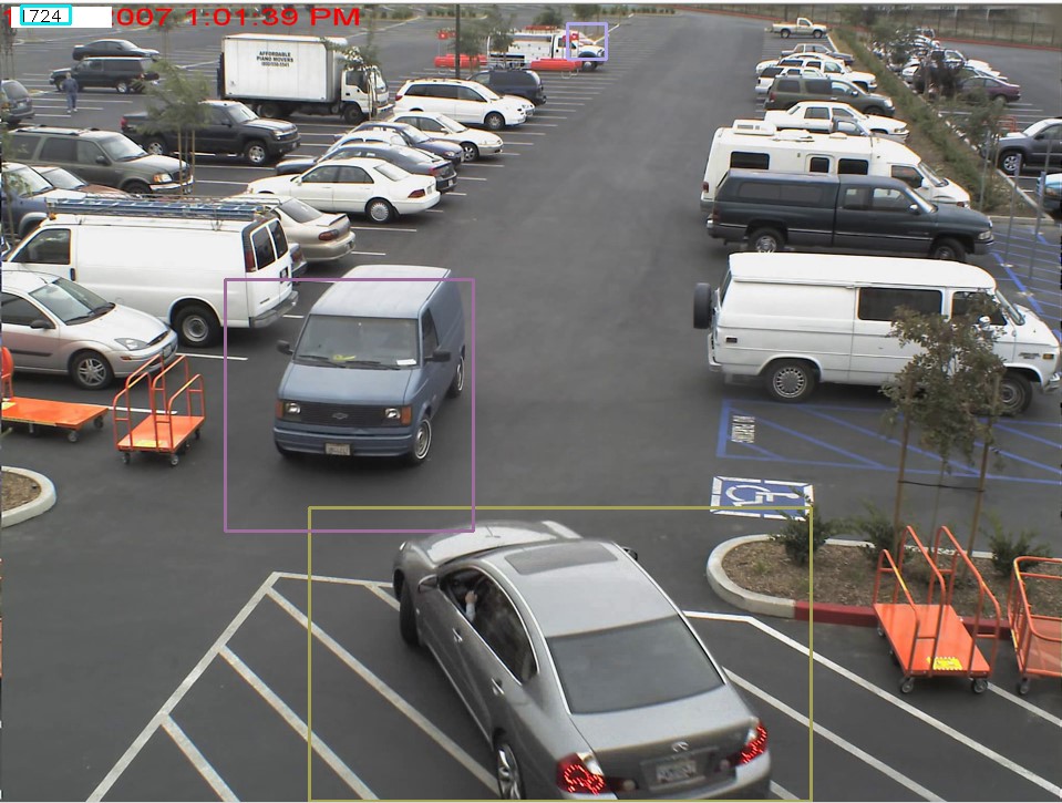
The goal of this project is to determine the state of a parking lot, more precisely the number of parking spaces. Basically this project is divided to two interconnected parts. One to determine number of parking spots from image, for example from first frame of video from camera, monitoring the parking lot, and second to determine wheter, or not is there a movement on the parking lot.

The process:

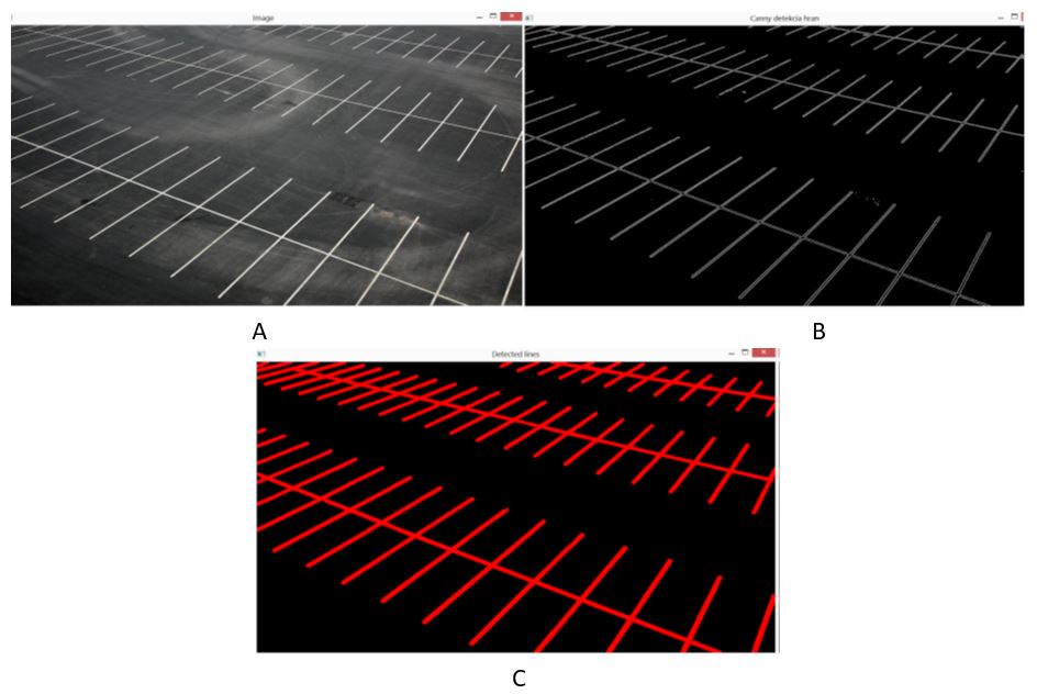
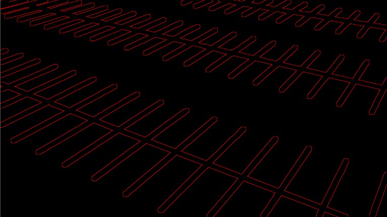
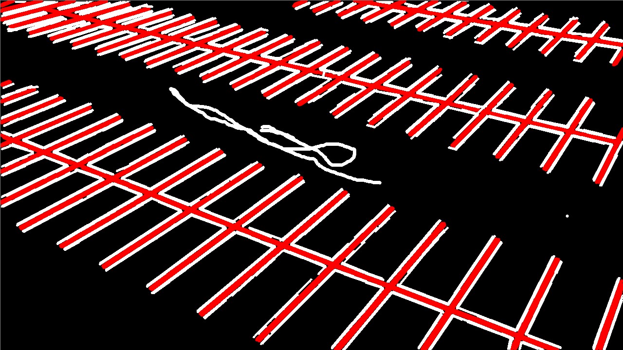
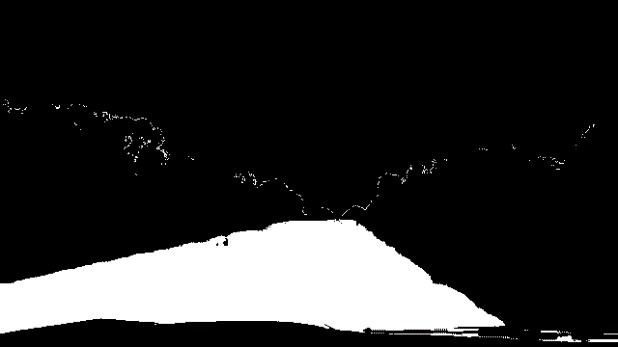
  1. We get parking lines from image of parking lot and get rid of noise:
    Canny(inputImage, helpMatrix, 450, 400, 3);
    cvtColor(helpMatrix, helpMatrix2, CV_GRAY2BGR);
    vector<Vec4i> lines;
    HoughLinesP(helpMatrix, lines, 1, CV_PI / 180, 7, 10, 10);
    for (size_t i = 0; i < lines.size(); i++)
    {
    	Vec4i l = lines[i];
    	line(helpMatrix2, Point(l[0], l[1]), Point(l[2], l[3]), Scalar(0, 0, 255), 5, CV_AA)
    }
    Mat element2 = getStructuringElement(CV_SHAPE_RECT, Size(3, 3));
    cv::erode(helpMatrix2, helpMatrix2, element);
    cv::dilate(helpMatrix2, helpMatrix2, element2);
    

    onder_edges
    Original Image (A), Canny edges with noise (B), HoughLines without noise (C)
  2. We use double dilate and substract their results to get mask of lines:
    morphologyEx(helpMatrix2, mark, CV_MOP_DILATE, element,Point(-1,-1), 3);
    morphologyEx(helpMatrix2, mark2, CV_MOP_DILATE, element, Point(-1, -1), 2);
    result = mark - mark2;
    

    onder_mask
    Result of dilating and substracting
  3. We use Canny and Hough lines, this time for removing the connecting line between each parking spot:
    Canny(resu, mark, 750, 800, 3);
    cvtColor(mark, mark2, CV_GRAY2BGR);
    mark2 = Scalar::all(0);
    vector<Vec4i> lines3;
    HoughLinesP(mark, lines3, 1, CV_PI / 180, 20, 15, 10);
    for (size_t i = 0; i < lines3.size(); i++)
    {
    	Vec4i l = lines3[i];
    	line(mark2, Point(l[0], l[1]), Point(l[2], l[3]), Scalar(0, 0, 255), 2, CV_AA);
    }
    

    onder_connection
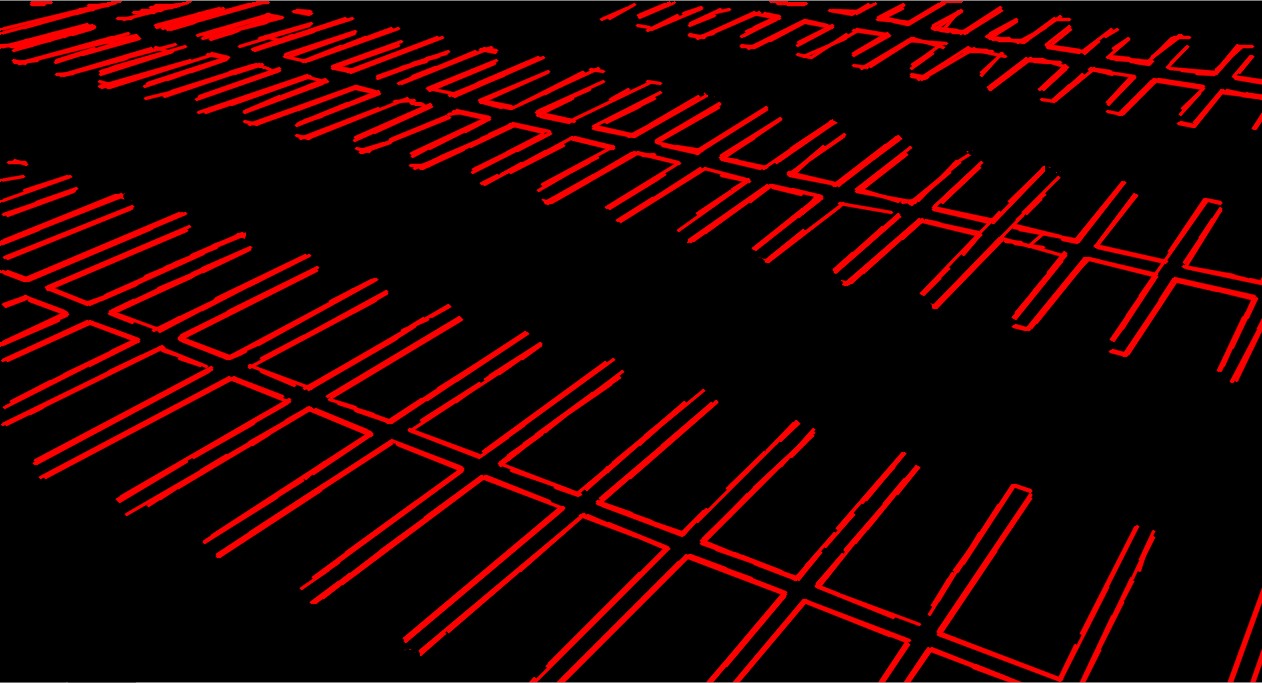
    Result of Hough lines to remove connection between lines in mask
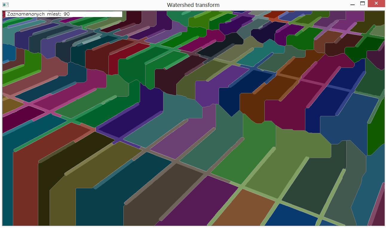
  4. We use this as a mask for finding contours for the Watershed algorithm and get result with detected parking spots, each colored with different color:
    vector<vector<Point> > contours;
    vector<Vec4i> hierarchy;
    findContours(markerMask, contours, hierarchy, RETR_CCOMP, CHAIN_APPROX_SIMPLE);
    int contourID = 0;
    for (; contourID >= 0; contourID = hierarchy[contourID][0], parkingSpaceCount++)
    {
    	drawContours(markers, contours, contourID, Scalar::all(parkingSpaceCount + 1), -1, 8, hierarchy, INT_MAX);
    }
    watershed(helpMatrix2, markers);
    Mat wshed(markers.size(), CV_8UC3);
    for (i = 0; i < markers.rows; i++)
    	for (j = 0; j < markers.cols; j++)
    	{
    		int index = markers.at<int>(i, j);
    		if (index == -1)
    			wshed.at<Vec3b>(i, j) = Vec3b(255, 255, 255);
    		else if (index <= 0 || index > parkingSpaceCount)
    			wshed.at<Vec3b>(i, j) = Vec3b(0, 0, 0);
    		else
    			wshed.at<Vec3b>(i, j) = colorTab[index - 1];
    	}
    

    onder_watershed
    Result of watershed algorithm with detected parking spots
  5. If our user is not satisfied with this result, he can always draw the seeds for watershed himself, or just adjust these seeds (img is the name of matrix, where user can see markers and markerMask matrix, where seeds are stored):
    Point prevPt(-1, -1);
    static void onMouse(int event, int x, int y, int flags, void*)
    {
    	if (event == EVENT_LBUTTONDOWN) prevPt = Point(x, y);
    	else if (event == EVENT_MOUSEMOVE && (flags & EVENT_FLAG_LBUTTON))
    	{
    		Point pt(x, y);
    		if (prevPt.x < 0)
    			prevPt = pt;
    		line(markerMask, prevPt, pt, Scalar::all(255), 5, 8, 0);
    		line(img, prevPt, pt, Scalar::all(255), 5, 8, 0);
    		prevPt = pt;
    		imshow("image", img);
    	}
    }
    

    onder_input_seeds
    User inputing seeds for watershed algorithm
  6. We have our spots stored, so we know their exact location, now its time to determine, wheter, or not check the lot again, if some vehicles are moving. For this purpose we need to detect movement on the lot with backgroundSubstraction, which can constantly learn what is static in image:
    Ptr<BackgroundSubtractor> pMOG2;
    pMOG2 = new BackgroundSubtractorMOG2(3000, 20.7,true);
    
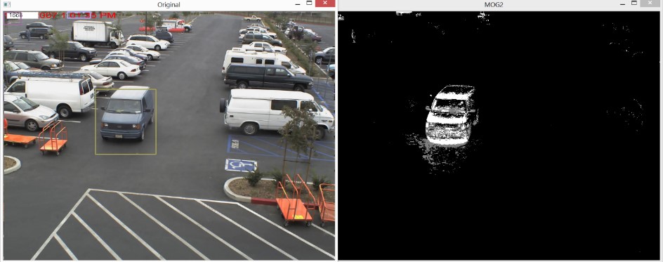
  7. We will give the MOG every frame captured from video feed and see what it results:
    pMOG2->operator()(frame, matMaskMog2,0.0035);
    imshow("MOG2", matMaskMog2);
    

    onder_MOG
    Result of MOG substraction
  8. As we can see, there is some noise detected – this noise represents for example moving leaves on trees, so it is necessary to remove it:
    cv::morphologyEx(matMaskMog2, matMaskMog2, CV_MOP_ERODE, element);
    cv::medianBlur(matMaskMog2, matMaskMog2, 3);
    cv::morphologyEx(matMaskMog2, matMaskMog2, CV_MOP_DILATE, element2);
    
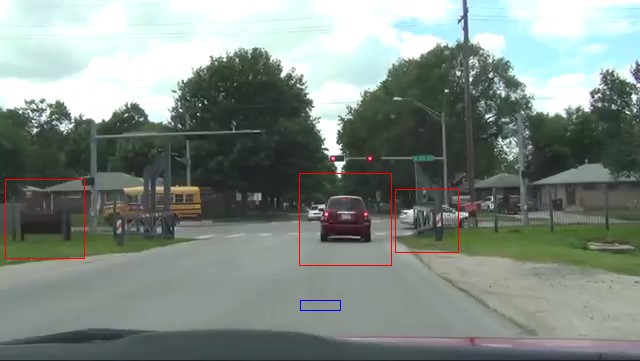
  9. Finally we find coordinates of moving object from MOG and draw a rectangle with random color around it (result can be seen at the top):
    scv::findContours(matMaskMog2, contours, CV_RETR_EXTERNAL, CV_CHAIN_APPROX_NONE);
    vector<vector<Point> > contours_poly(contours.size());
    vector<Rect> boundRect(contours.size());
    
    for (int i = 0; i < contours.size(); i++)
    {
    approxPolyDP(Mat(contours[i]), contours_poly[i], 3, true);
    	boundRect[i] = boundingRect(Mat(contours_poly[i]));		
    }
    RNG rng(01);
    for (int i = 0; i< contours.size(); i++)
    {
    Scalar color = Scalar(rng.uniform(0, 255), rng.uniform(0, 255), rng.uniform(0, 255)); 
    	rectangle(frame, boundRect[i].tl(), boundRect[i].br(), color, 2, 8, 0);
    }
    

Result:

We have a functional parking spot detection, which means we can easily determine how much parking spots our parking lot have. We also have stored where are these parking spots exactly located. From the camera feed, we can detect car movement and also determine, on which coordinates the movement stopped. We did not implemented the function to connect these infomormation sources, but it can be easily added.

Limitations:

  • For parking spots detection we need an empty lot. Otherwise it will be nearly impossible to determine where are these spots exactly located, mainly if vehicles are not parking at their exact center.
  • For movement detection, we need static camera feed, becouse of used MOG method, which constantly learns what is background and which object are moving.
  • Parking spots detection is not perfect, it still needs some user correction to determine exact number of parking spots.
Posted on

Car detection in videos

Peter Horvath

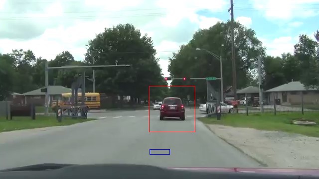
We detect cars from videos recorded by dash cameras situated in cars. This type of camera is dynamic so we decided to train and use Haar Cascade Classifier. The classifier itself returns a lot of false positive results. So we improved classifier by removing false positive results using road detection.

Functions used: cvtColor, split, Rect, inRange, equalizeHist, detectMultiScale, rectangle, bitwise_and

Process

1st part – training haar cascade classifier

Collect a set of positive samples and negative samples. Make a list file of both (positives.dat and negatives.dat). Then use opencv_createsamples function with parameters to make a single .vec file with all positive samples.

opencv_createsamples -info positives.dat -vec samples.vec -num 500 -w 20 -h 20

Now train a cascade classifier using HAAR features

opencv_traincascade -data classifier -featureType HAAR -vec samples.vec -bg negatives.dat -numPos 500 -numNeg 850 -numStages 15 -precalcValBufSize 1000 -precalcIdxBufSize 1000 -minHitRate 0.999 -maxFalseAlarmRate 0.5 -mode ALL -w 20 -h 20

Output of this procedure is trained classifier – xml file.

2nd part – using classifier in C++ code to detect cars, improved by road detection

Open video file using VideoCapture. For every video frame do:

  1. Convert actual video frame to HSV color model
    cvtColor(frame, frame_hsv, CV_BGR2HSV);
    
  2. Make sum of H S V in captured road sample. Calculate average Hue Saturation and Value of captured road sample.
    int averageHue = sumHue / (rectangle_hsv_channels[0].rows*rectangle_hsv_channels[0].cols);
    int averageSat = sumSat / (rectangle_hsv_channels[1].rows*rectangle_hsv_channels[1].cols);
    int averageVal = sumVal / (rectangle_hsv_channels[2].rows*rectangle_hsv_channels[2].cols);
    
  3. Use inRange function to make a binary result – road is white colored, other is black colored
    inRange(frame_hsv, cv::Scalar(averageHue - 180, averageSat - 15, averageVal - 20), cv::Scalar(averageHue + 180, averageSat + 15, averageVal + 20), final);		
    

    horvath_binary

  4. Convert actual video frame to grayscale
    cvtColor(frame, image_gray, CV_BGR2GRAY);
    
  5. Create an instance of CascadeClassifier
    String car_cascade_file = "classifier.xml";
    CascadeClassifier car_classifier;
    car_classifier.load(car_cascade_file);
    
  6. Detect cars in grayscale video frame using classifier
    car_classifier.detectMultiScale(image_gray, cars, 1.1, 2, 0 | CV_HAAR_SCALE_IMAGE, Size(20, 20));
    

    Result have a lot of false positives

    horvath_false_positives

  7. Make a black image with white squares at locations returned by cascade classifier. Make logical and between it and image with detected road
    horvath_filter
  8. Accept only squares which have at least 20% of pixels white.
    horvath_result

Limitations:

  • Cascade classifier trained only with 560 positive and 860 negative samples – detect cars only from near distance
  • Road detection fails when some object (car, road line) comes to blue rectangle (supposed to be road sample)
  • Dirt have a similar saturation as road – detected as road
Posted on

Card detection

Michael Garaj

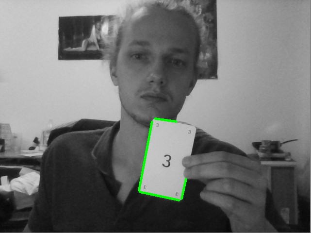
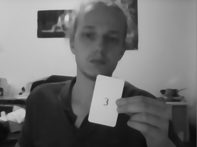
The goal of this project is to detect card in captured image. Motivation was to make automatized recognizer of cards for poker tournaments. Application is implemented to find orthogonal edges in an image and try to find card by ratio of its edges.

Process of finding and recognizing a card in image follows these steps:

  1. Load an image from local repository.
  2. Apply blur and bilateral filter.
    garaj_blur
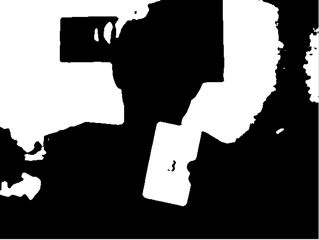
  3. Compute binary threshold.
    garaj_threshold
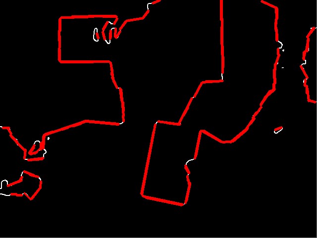
  4. Extract edges from binary image by Canny algorithm.
  5. Apply Hough lines to get lines find in edge image.
    garaj_hough_lines
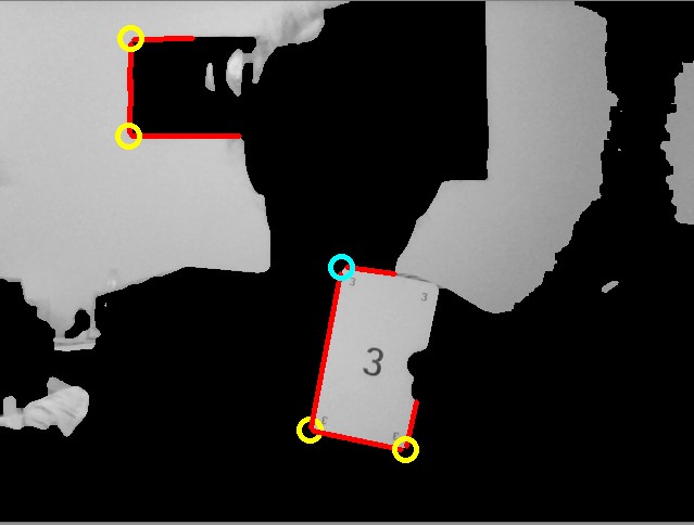
  6. Search for orthogonal lines and store them in structure for future optimalization.
  7. Optimise number of detected lines in same area by choosing only the biggest ones.
    garaj_optimised_lines
  8. Find card which consist of 3 touching lines.
  9. Compute ratio of the lines and identify cards in the image.
    garaj_identification
    Following code sample shows steps of optimalization of detected corners:

    vector<MyCorner> optimalize(vector<MyCorner> corners, Mat image) {
    	vector<MyCorner> optCorners;
    
    	for (int i = 0; i < corners.size(); i++) {
    		corners[i].crossing = crossLines(corners[i]);
    		corners[i].single = 1;
    	}
    
    	int distance = 25;
    	for (int i = 0; i < corners.size() - 1; i++) {
    		MyCorner corner = corners[i];
    		float lengthI = 0, lengthJ = 0;
    
    		if (corner.single){
    			for (int j = i + 1; j < corners.size(); j++) {
    
    				if (abs(corner.crossing.x - corners[j].crossing.x) < distance && abs(corner.crossing.y - corners[j].crossing.y) < distance &&
    					(corner.single || corners[j].single)) {
    
    					lengthI = getLength(corner.u) + getLength(corner.v);
    					lengthJ = getLength(corners[j].u) + getLength(corners[j].v);
    
    					if (lengthI < lengthJ) {
    						corner = corners[j];
    					}
    					corner.single = 0;
    					corners[i].single = 0;
    					corners[j].single = 0;
    				}
    			}
    			optCorners.push_back(corner);
    		}
    	}
    
    	return optCorners;
    }
    
Posted on

Bag of Words algorithm

Tomas Drutarovsky

We implement well-known Bag of Words algorithm (BoW) in order to perform image classification of tiger cat images. In the work, we use a subset of publicly available ImageNet dataset and divide data on two sets – tiger cats and non-cat objects, which consist of images of 10 random chosen object types.

The main processing algorithm is performed by these steps:

  1. Choose a suitable subset of images from a large dataset
    • We use around 100 000 unique images
  2. Detect keypoints
    • We detect keypoints using SIFT or Dense keypoint extractor
    DenseFeatureDetector dense(20.0f, 3, 2, 10, 4);
    BOWKMeansTrainer bowTrainer(dictionarySize, tc, retries, flags);
    
    for (int i = 0; i < list.count(); i++){
    	Mat img = imread(list.at(i), CV_LOAD_IMAGE_COLOR);
    
    	dense.detect(img, keypoints);
    }
    

    drutarovsky_keypoints
    Keypoints detected using SIFT detect function – more than 500 keypoints.
  3. Describe keypoints using SIFT
    • SIFT descriptor produces description for each keypoint separately
      sift.compute(img, keypoints, descriptor);
      bowTrainer.add(descriptor);
      
  4. Cluster descriptors using k-means
    • Around 10 million of keypoints are chosen to cluster
    • Clustering results in 1000 clusters represented by centroids (visual words)
    Mat vocabulary = bowTrainer.cluster();
    
  5. Calculate BoW descriptors
    • Each keypoint from an input image is then evaluated for response from 1000 visual words or represents
    • Histogram of reponse is normalized for each image
    Ptr<DescriptorMatcher> matcher(new FlannBasedMatcher);
    Ptr<FeatureDetector> detector(new SiftFeatureDetector());
    BOWImgDescriptorExtractor bowExtractor(detector, matcher);
    bowExtractor.compute(img, keypoints, descriptor);
    

    drutarovsky_BoW_descriptor
    BoW descriptor of 200 ats visualized over 1000 clustered visual words vocabulary
  6. Train SVM using BoW descriptors
    • Calculated histograms or BoW descriptors are trained using linear SVM
    • Suitable rate between positive and negative subset needs to be chosen
  7. Test images using SVM
    • Response of test images is used to evaluate algorithm
    • Our model shows accuracy of (62% of positive set and 58% of negative set)
    • Better results are achievable using larger datasets, but both time and computational power are necessary
Posted on

Detection of objects in soccer

Lukas Sekerak

Project idea

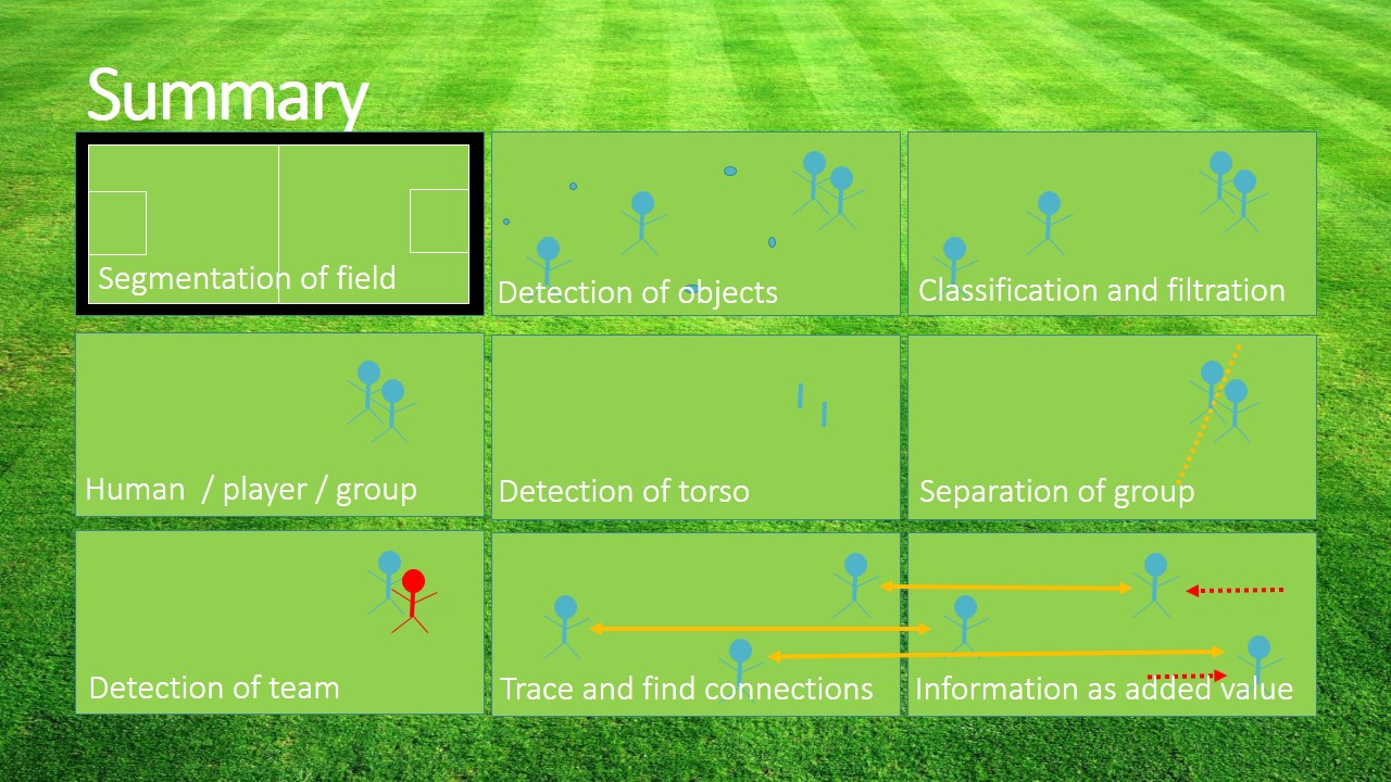
Try detect objects (players, soccer ball, referees, goal keeper) in soccer match. Detect their position, movement and show picked object in ROI area. More info in a presentation and description document.

Requirements

  • Opencv 2.4
  • log4cpp

Dataset videos

Operation Agreement CNR-FIGC

T. D’Orazio, M.Leo, N. Mosca, P.Spagnolo, P.L.Mazzeo A Semi-Automatic System for Ground Truth Generation of Soccer Video Sequences in the Proceeding of the 6th IEEE International Conference on Advanced Video and Signal Surveillance, Genoa, Italy September 2-4 2009

Setup

  1. Clone this repository into workspace
  2. Download external requirements + dataset
  3. Build project
  4. Run project

Control keys

  • W – turn on/off ROI area
  • Q,E – switch between detected ROI
  • S – pause of processing frames
  • F – turn on/off debug draw

License

This software is released under the MIT License.

Credits

  • Ing. Wanda BeneÅ¡ová, PhD. – Supervisor

2


Project repository: https://github.com/sekys/sk.seky.soccerball

Posted on

Object removing in image/video

Marek Grznar

Introduction

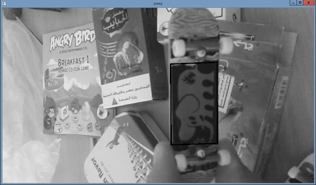
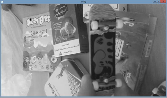
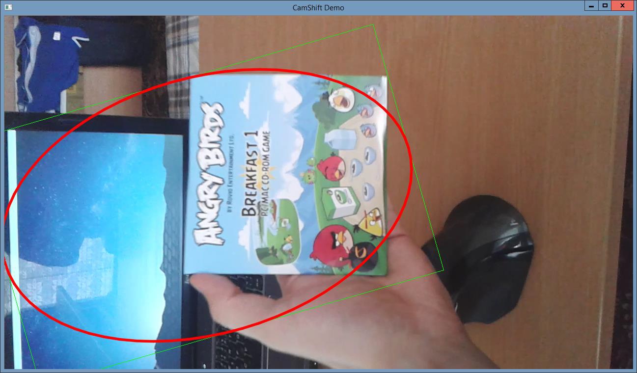
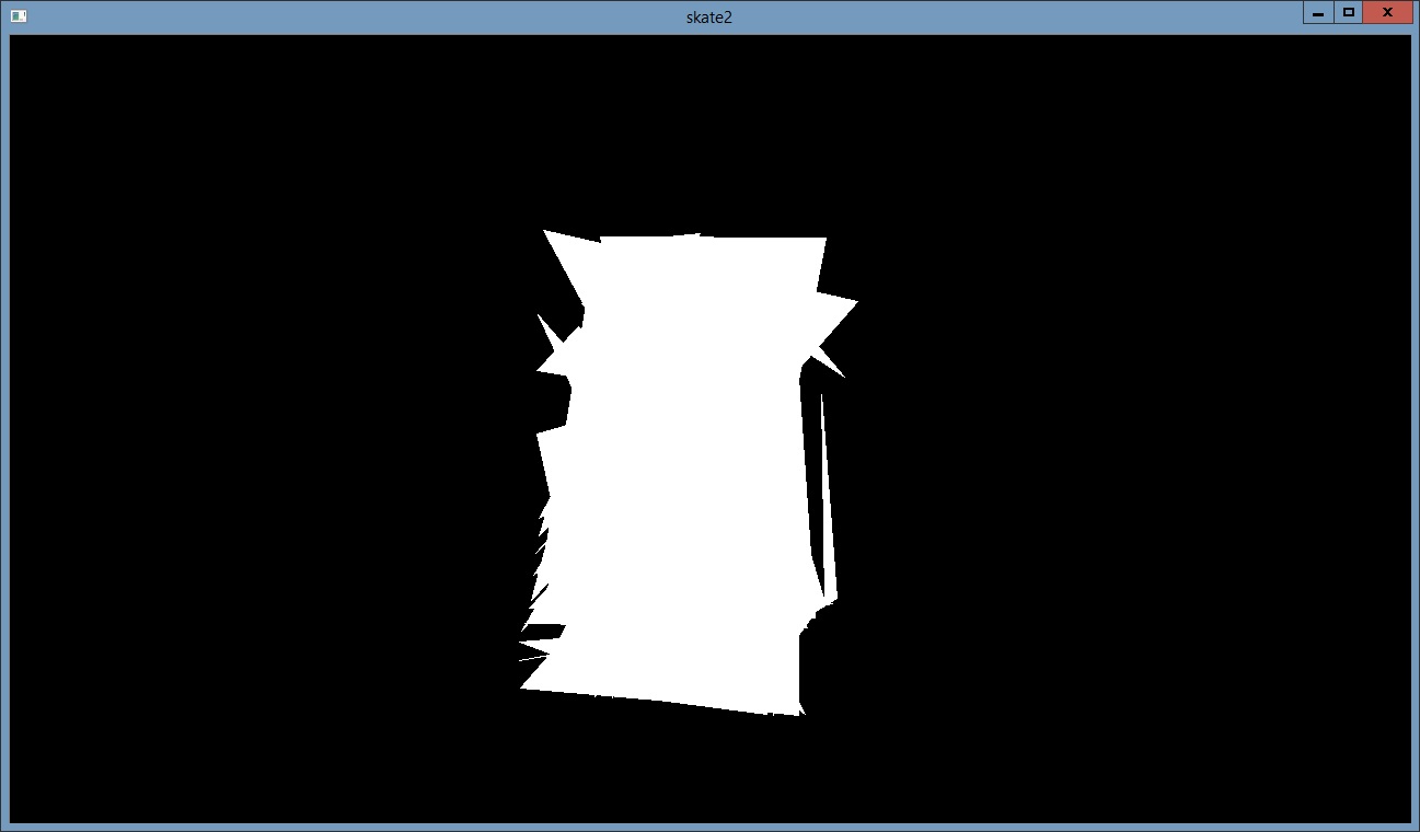
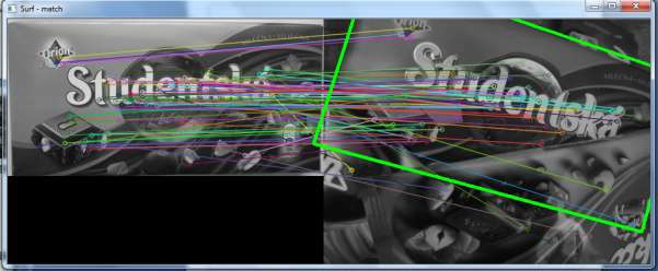
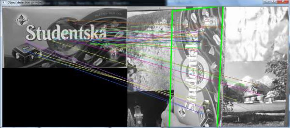
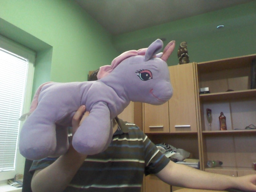
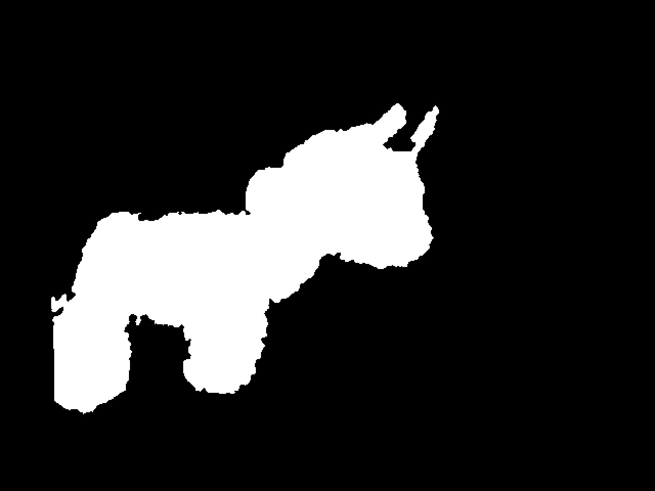
In our project we focus on simple object recognition, then tracking this recognized object and finally we try to delete this object from video. By object recognition we used local features-based methods. We compare SIFT and SURF methods for detection and description. By RANSAC algorithm we compute the homography. In case these algorithms successfully find the object we create a mask where recognized object was white area and the rest was black. By object tracking we compared the two approaches. The first approach is based on calculating optical flow using the iterative Lucas-Kanade method with pyramids. The second approach is based on camshift tracking algorithm. For deleting the object from video we focus to using algorithm based on restoring the selected region in an image using the region neighborhood.

Used functions: floodFill, findHomography, match, fillPoly, goodFeaturesToTrack, calcOpticalFlowPyrLK, inpaint, mixChannels, calcHist, CamShift

Solution

  1. Opening video file, retrieve the next frame (picture), converting from color image to grayscale
    cap.open("Video1.mp4");
    cap >> frame; 
    frame.copyTo(image); 
    cvtColor(image, gray, COLOR_BGR2GRAY);
    
  2. Find object in frame (picture)
    1. Keypoints detection and description (SIFT/SURF)
      // SiftFeatureDetector detector( minHessian ); 
      SurfFeatureDetector detector( minHessian );
      
      std::vector<KeyPoint> keypoints_object, keypoints_scene;
      
      detector.detect(img_object, keypoints_object); 
      detector.detect(img_scene, keypoints_scene);
      
      // SiftDescriptorExtractor extractor; 
      SurfDescriptorExtractor extractor;
      
      Mat descriptors_object, descriptors_scene;
      
      extractor.compute(img_object, keypoints_object, descriptors_object); 
      extractor.compute(img_scene, keypoints_scene, descriptors_scene);
      
    2. Matching keypoints
      FlannBasedMatcher matcher;
      std::vector< DMatch > matches; 
      matcher.match( descriptors_object, descriptors_scene, matches );
      
    3. Homography calculating
      Mat H = findHomography( obj, scene, CV_RANSAC );
      
    4. Mask creating
      cv::Mat mask(img_scene.size().height,img_scene.size().width,CV_8UC1);
      mask.setTo(Scalar::all(0));
      cv::fillPoly(mask,&pts, &n, 1, Scalar::all(255));
      

First tracking approach

  1. Find significant points in current frame (using mask with recognized object)
  2. Find significant points from the previous frame to the next
  3. Deleting object from image
    1. Calculate mask of current object position
    2. Modify mask of current object position
    3. Restore the selected region in an image using the region neighborhood.

Second tracking approach

  1. Calculate histogram of ROI
  2. Calculate the back projection of histogram
  3. Track object using camshift

Object recognition

Input

grznar_input

Outputs

grznar_surf
Surf (recognized object is in black rectangle)
grznar_sift
Sift (black dot is recognized object)

Tracking object

Input (tracked object)

grznar_input2

Outputs

grznar_approach1
first approach
grznar_approach2
Second approach

Modifying mask for deleting object

Input

grznar_mask1

Output

grznar_mask2

Deleting object

Input

grznar_input3

Output

Object_remove

Posted on

Local Descriptors in OpenCv

Tomas Martinkovic

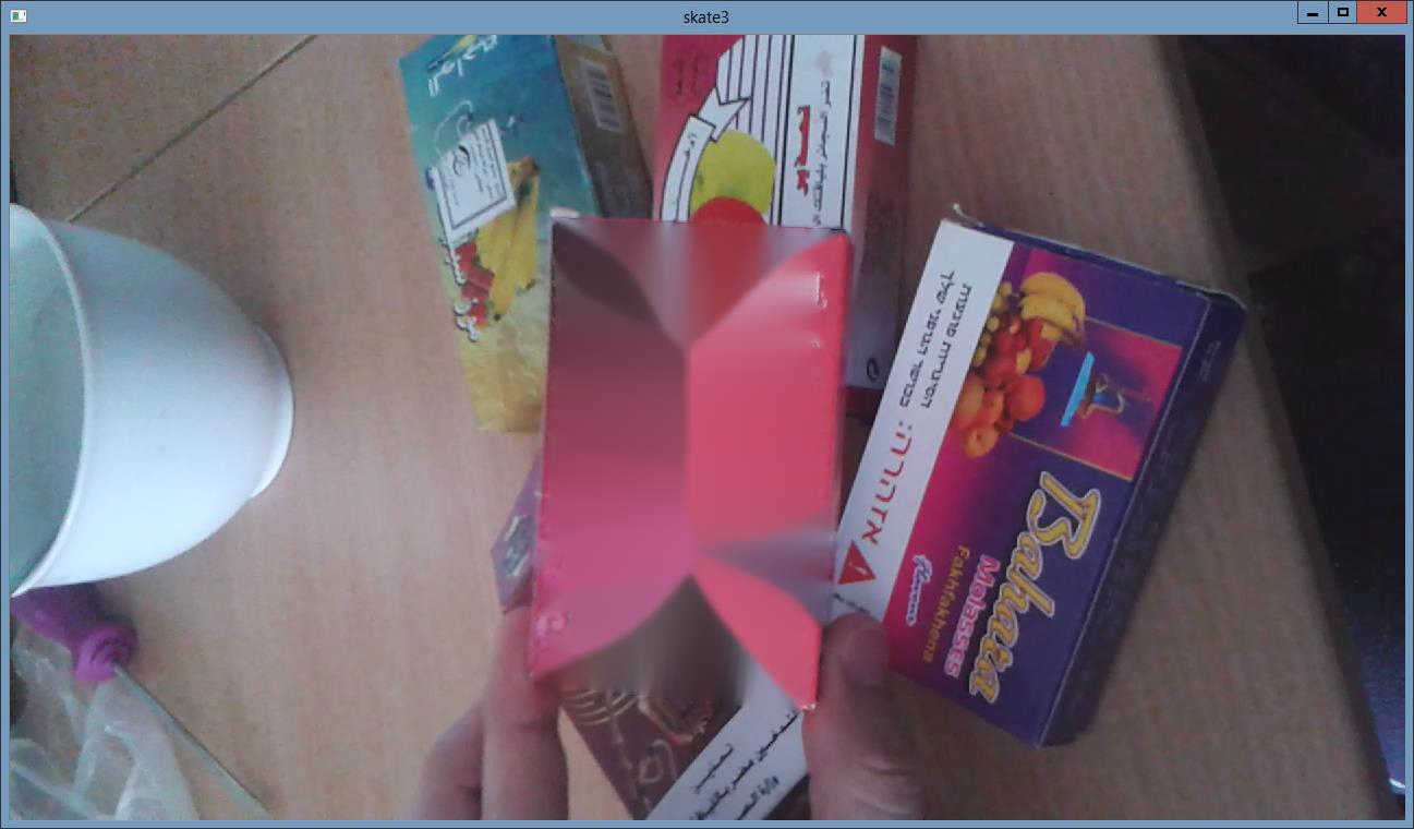
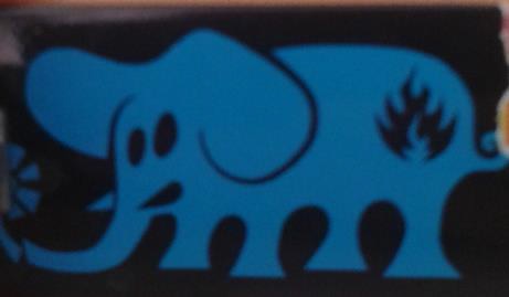
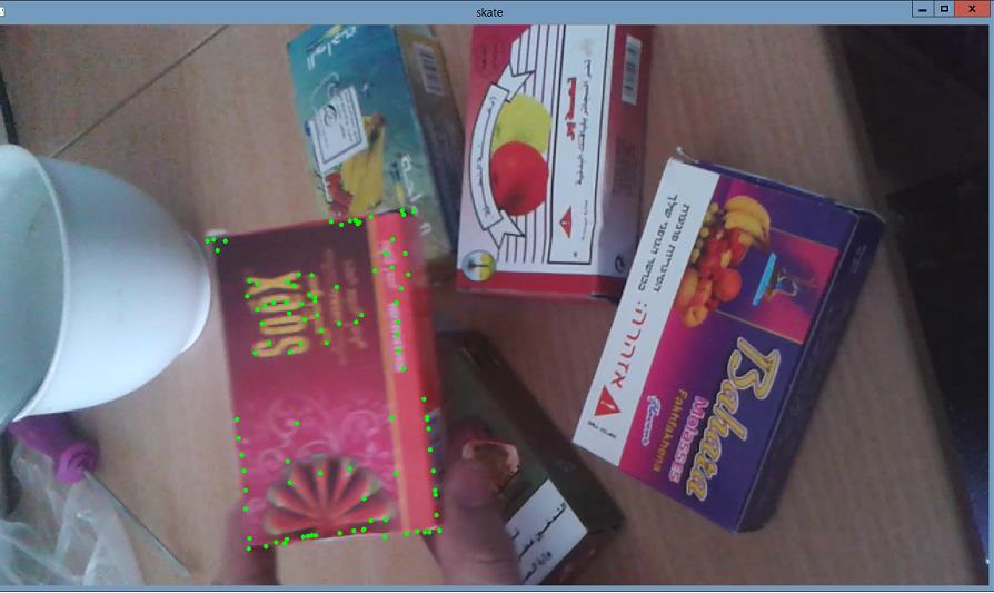
The project shows detection of chocolate cover from input image or frame of video. For each video or image may be chosen various combinations of detector with descriptor. For matching object of chocolate cover with input frame or image automatically is used FlannBasedMatcher or BruteForceMatcher. It depends on the chosen SurfDescriptorExtractor or FREAK algorithm.

Functions used: SurfFeatureDetector, FastFeatureDetector, SiftFeatureDetector, StarFeatureDetector, SurfDescriptorExtractor, FREAK, FlannBasedMatcher, BruteForceMatcher, findHomography

Process

  1. Preprocessing – Conversion to grayscale
    cvtColor(frame, img_scene, CV_BGR2GRAY);
    
  2. Detect the keypoints
    detector_Surf = getSurfFeatureDetector();
    detector_Surf.detect( img_object, keypoints_object );
    detector_Surf.detect( img_scene, keypoints_scene );
    
  3. Compute local descriptors
    extractor_freak.compute( img_object, keypoints_object, descriptors_object );
    extractor_freak.compute( img_scene, keypoints_scene, descriptors_scene );
    
  4. Matching local descriptors
    BruteForceMatcher<Hamming> matcher;
    matcher.match( descriptors_object, descriptors_scene, matches );
    
  5. Draw good matches to frame
    drawMatches( img_object, keypoints_object, img_scene, keypoints_scene, good_matches, img_matches, Scalar::all(-1), Scalar::all(-1), vector<char>(), DrawMatchesFlags::NOT_DRAW_SINGLE_POINTS );
    
  6. Finding homography and drawing frame of video
    Mat H = findHomography( obj, scene, CV_RANSAC );
    perspectiveTransform( obj_corners, scene_corners, H);
    imshow( "Object detection on video", img_matches );
    

Sample

Martinkovic
Matching local descriptors in the image.
Martinkovic2
Matching local descriptors in the video.
Posted on

Smile detection

Jan Podmajersky

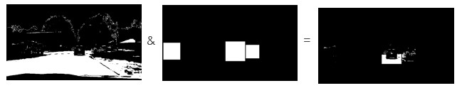
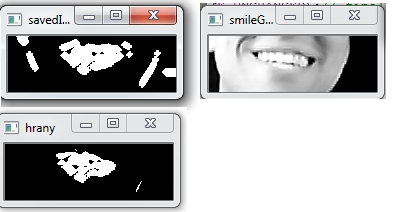
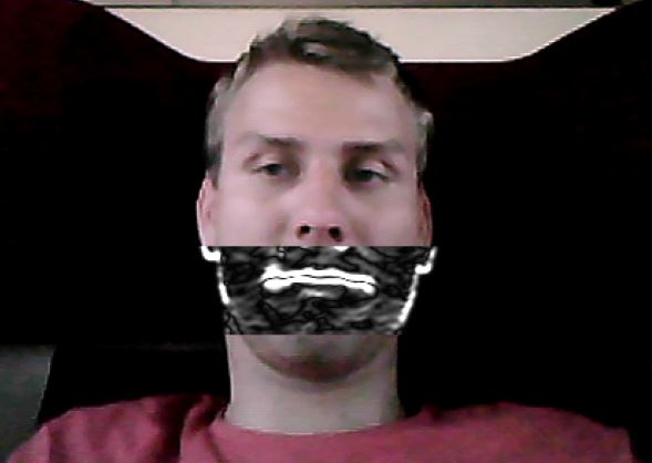
Smile detection is a popular feature of today’s photo cameras. It is not implemented in all cameras, as a popular face detection, because it is more complicated to implement. This project shows a basic algorihtm in the topic. It may be used but few improvements are necessary. Sobel filter and thresholding are used. There is a mask which is compared to every filtered image from a webcam. If the images are more than 60% equal, smile is detected.
Used Functions detectMultiScale, Sobel, medianBlur, threshold, dilate, bitwise_and

The process

  1. convert image from camera to gray scale
    cvtColor( frame, frame_gray, CV_BGR2GRAY );
    
  2. face detection using Haar cascade
    face_cascade.detectMultiScale( frame_gray, faces, 1.3, 4, CV_HAAR_DO_CANNY_PRUNING, Size(50, 50) );
    
  3. adjust size of image just to the detected face
  4. cut only one third of the face, where mouth are always located
    face = frame_gray( cv::Rect(faces[i].x, faces[i].y + 2 * faces[i].height/3, faces[i].width, faces[i].height/3) );
    
  5. horizontal sobel filter
    Sobel( face, grad_y, ddepth, 0, 1, 7, scale, delta, BORDER_DEFAULT );
    addWeighted( abs_grad_y, 0.9, abs_grad_y, 0.9, 0, output );
    
  6. Median blur
    medianBlur(output, detected_edges, 5);
    
  7. threshold the image
    threshold(detected_edges, detected_edges, 220, 255, CV_THRESH_BINARY);
    
  8. dilate small parts
    dilate(detected_edges, detected_edges, element);
    
  9. logical and the image and mask image
    bitwise_and(detected_edges,maskImage,result);
    
  10. detect smile
    if the images are 60% equal there is a smile
podmajersky_input
input
podmajersky_sobel
horizontal Sobel filter
Podmajersky_smile
masked image
podmajersky_output
output
Posted on

SIFT in RGB-D (Object recognition)

Marek Jakab

In this example we focus on enhancing the current SIFT descriptor vector with additional two dimensions using depth map information obtained from kinect device. Depth map is used for object segmentation (see: http://vgg.fiit.stuba.sk/2013-07/object-segmentation/) as well to compute standard deviation and the difference of minimal and maximal distance from surface around each of detected keypoints. Those two metrics are used to enhance SIFT descriptor.

Functions used: FeatureDetector::detect, DescriptorExtractor::compute, RangeImage∷calculate3DPoint

The process

For extracting normal vector and compute mentioned metrics from the keypoint we use OpenCV and PCL library. We are performing selected steps:

  1. Perform SIFT keypoint localization at selected image & mask
  2. Extract SIFT descriptors
    // Detect features and extract descriptors from object intensity image.
    if (siftGpu.empty())
    {
    	featureDetector->detect(intensityImage, objectKeypoints, mask);
    	descriptorExtractor->compute(intensityImage, objectKeypoints, objectDescriptors);
    }
    else
    {
    	runSiftGpu(siftGpu, maskedIntensityImage, objectKeypoints, objectDescriptors, mask);
    }
    
    
  3. For each descriptor
    1. From surface around keypoint position:
      1. Compute standard deviation
      2. Compute difference of minimal and maximal distances (based on normal vector)
    2. Append new information to current descriptor vector
    for (int i = 0; i < keypoints.size(); ++i)
    {
    	if (!rangeImage.isValid((int)keypoints[i].x, (int)keypoints[i].y))
    	{
    		setNullDescriptor(descriptor);
    		continue;
    	}
    	rangeImage.calculate3DPoint(keypoints[i].x, keypoints[i].y, point_in_image.range, keypointPosition);
    	sufraceSegmentPixels = rangeImage.getInterpolatedSurfaceProjection(transformation, segmentPixelSize, segmentWorldSize);
    	rangeImage.getNormal((int)keypoints[i].x, (int)keypoints[i].y, 5, normal);
    	for (int j = 0; j < segmentPixelsTotal; ++j)
    	{
    		if (!pcl_isfinite(sufraceSegmentPixels[j]))
    			sufraceSegmentPixels[j] = maxDistance;
    	}
    	cv::Mat surfaceSegment(segmentPixelSize, segmentPixelSize, CV_32FC1, (void *)sufraceSegmentPixels);
    	extractDescriptor(surfaceSegment, descriptor);
    }
    
    
    void DepthDescriptor::extractDescriptor(const cv::Mat &segmentSurface, float *descriptor)
    {
    	cv::Scalar mean;
    	cv::Scalar standardDeviation;
    	meanStdDev(segmentSurface, mean, standardDeviation);
    
    	double min, max;
    	minMaxLoc(segmentSurface, &min, &max);
    
    	descriptor[0] = float(standardDeviation[0]);
    	descriptor[1] = float(max - min);
    }


Inputs

jakab_input
The color image
jakab_mask
The mask from segmented object.

Output

To be able to enhance SIFT descriptor and still provide good matching results, we need to evaluate the precision of selected metrics. We have chosen to visualize the normal vectors computed from the surface around keypoints.

jakab_output
Normal vector visualisation
Posted on

Fire detection in video

Stefan Linner

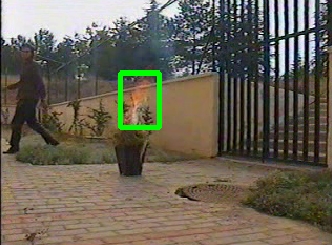
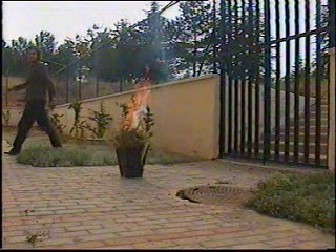
The main aim of this example is to automatically detect fire in video, using computer vision methods, implemented in real-time with the aid of the OpenCV library. Proposed solution must be applicable in existing security systems, meaning with the use of regular industrial or personal video cameras. Necessary solution precondition is that camera is static. Given the computer vision and image processing point of view, stated problem corresponds to detection of dynamically changing object, based on his color and moving features.

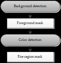
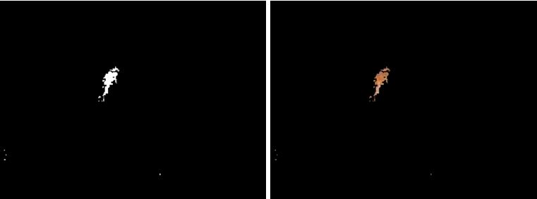
While static cameras are utilized, background detection method provides effective segmentation of dynamic objects in video sequence. Candidate fire-like regions of segmented foreground objects are determined according to the rule-based color detection.
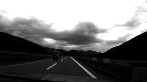
Input

linner_input

Process outline

linner_process

Process steps

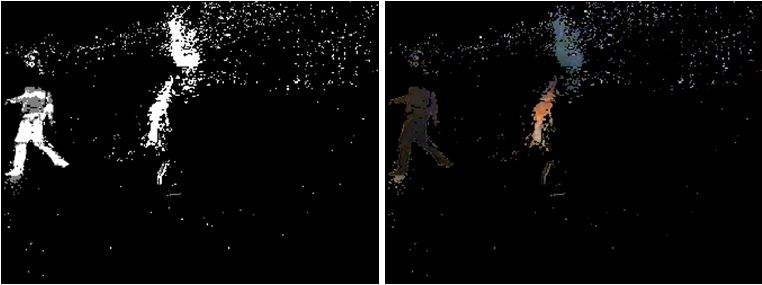
  1. Retrieve current video frame
    capture.retrieve(frame);
    
  2. Update background model and save foreground mask to
    BackgroundSubtractorMOG2 pMOG2;
    Mat fgMaskMOG2,
    pMOG2(frame, fgMaskMOG2);
    
  3. Convert current 8-bit frame in RGB color space to 32-bit floating point YCbCr color space.
    frame.convertTo(temp, CV_32FC3, 1/255.0);
    cvtColor(temp, imageYCrCb, CV_BGR2YCrCb);
    
  4. For every frame pixel, check if it is foreground and if it meets the expected fire color features.
    colorMask = Mat(frame.rows, frame.cols, CV_8UC1);
    for (int i = 0; i < imageYCrCb.rows; i++){
    	const uchar* fgMaskValuePt = fgMaskMOG2.ptr<uchar>(i);
    	uchar* colorMaskValuePt = colorMask.ptr<uchar>(i);
    	for (int j = 0; j < imageYCrCb.cols; j++){ if (fgMaskMOG2[j] > 0 && isFirePixel(i, j))
    			colorMaskValuePt[j] = 255;
    		else
    			colorMaskValuePt[j] = 0;
    	}
    }
    
    …
    
    const int COLOR_DETECTION_THRESHOLD = 40;
    bool isFirePixel(const int row, const int column){
    	…
    		if (valueY > valueCb
    			&& intValueCr > intValueCb
    			&& (valueY > meanY && valueCb < meanCb && valueCr > meanCr)
    			&& ((abs(valueCb - valueCr) * 255) > COLOR_DETECTION_THRESHOLD))
    			return true;
    
  5. Draw bounding rectangle
    vector<Point> firePixels;
    …
    if (colorMaskPt[j] > 0)
    firePixels.push_back(Point(j, i));
    …
    rectangle(frame, boundingRect(firePixels), Scalar(0, 255, 0), 4, 1, 0);
    

Samples

linner_mask
Foreground mask
linner_mask2
Fire region mask
Linner_Fire
Result

References

CELIK, T., DEMIREL, H.: Fire detection in video sequences using a generic color model. In: Fire Safety Journal, 2008, 44.2: 147-158.

Posted on

Eye-Shape Classification

Veronika Štrbáková

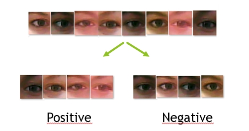
The project shows detection and recognition of face and eyes from input image (webcam). I use for detection and classification haarcascade files from OpenCV. If eyes are recognized, I classify them as opened or narrowed. The algorithm uses the OpenCV and SVMLight library.

Functions used: CascadeClassifier::detectMultiScale, HOGDescriptor::compute HOGDescriptor::setSVMDetector, SVMTrainer::writeFeatureVectorToFile

The process:

  1. As first I make positive and negative dataset. Positive dataset are photos of narrowed eyes and negative dataset are photos of opened eyes.
    Strbakova_eye
  2. Then I make HOGDescriptor and I use it to compute feature vector for every picture. These pictures are used to train SVM vector and their feature vectors are saved to one file: features.dat
    HOGDescriptor hog;
    vector<float> featureVector;
    SVMLight::SVMTrainer svm("features.dat");
    hog.compute(img, featureVector, Size(8, 8), Size(0, 0));
    svm.writeFeatureVectorToFile(featureVector, true);
    
  3. From feature vectors I compute single descriptor vector and I set him to my HOGDescriptor.
    SVMLight::SVMClassifier c("classifier.dat");
    vector descriptorVector = c.getDescriptorVector();
    hog.setSVMDetector(descriptorVector);
    
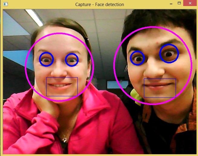
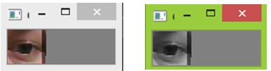
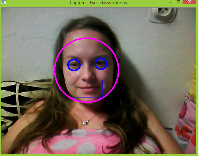
  4. I detect every face and every eye from picture. For every found picture of eye I cut it and I use HOGDescriptor to detect narrowed shape of eye.
    strbakova_face_det
    Face, Eye and Mouth detection
    strbakova_cutting_eyes
    Cutting eyes and conversion to grayscale format

    strbakova_narrowed_eyes.jpg
    Finding narrowed eyes