Posted on

Exploring Visual Saliency of Real Objects at Different Depths

Depth cues are important aspects that influence the visual saliency of objects around us. However, the depth aspect and its quantified impact on the visual saliency has not yet been thoroughly examined in real environments. We designed and carried out an experimental study to examine the influence of the depth cues on the visual saliency of the objects at the scene. The experimental study took place with 28 participants under laboratory conditions with the objects in various depth configurations at the real scene. Visual attention data were measured by the wearable eye-tracking glasses. .. more

Posted on

Color Saliency

Color is a fundamental component of visual attention. Saliency is usually associated with color contrasts. Besides this bottom-up perspective, some recent works indicate that psychological aspects should be considered too. However, relatively little research has been done on the potential impacts of color psychology on attention. To our best knowledge, a publicly available fixation dataset specialized in color features does not exist. We, therefore, conducted a novel eye-tracking experiment with color stimuli. We studied  fixations of 15 participants to find out whether color differences can reliably model color saliency or particular colors are preferably fixated regardless of scene content, i.e. color prior. … more


Posted on

Effects of individual’s emotions on saliency and visual search

Patrik Polatsek, Miroslav Laco, Šimon Dekrét, Wanda Benesova, Martina Baránková, Bronislava Strnádelová, Jana Koróniová, Mária Gablíková

Abstract.

While psychological studies have confirmed a connection between emotional stimuli and visual attention, there is a lack of evidence, how much influence individual’s mood has on visual information processing of emotionally neutral stimuli. In contrast to prior studies, we explored if bottom-up low-level saliency could be affected by positive mood. We therefore induced positive or neutral emotions in 10 subjects using autobiographical memories during free-viewing, memorizing the image content and three visual search tasks. We explored differences in human gaze behavior between both emotions and relate their fixations with bottom-up saliency predicted by a traditional computational model. We observed that positive emotions produce a stronger saliency effect only during free exploration of valence-neutral stimuli. However, the opposite effect was observed during task-based analysis. We also found that tasks could be solved less efficiently when experiencing a positive mood and therefore, we suggest that it rather distracts users from a task.

download: saliency-emotions

Please cite this paper if you use the dataset:

Polatsek, P., Laco, M., Dekrét, Š., Benesova, W., Baránková, M., Strnádelová, B., Koróniová, J., & Gablíková, M. (2019)

Effects of individual’s emotions on saliency and visual search

Posted on

Camera tracking

Martin Volovar

Camera tracking is used in visual effects to synchronize movement and rotation between real and virtual camera .This article deals with obtaining rotation and translation from two images and trying to reconstruct scene.

  1. First we need find keypoints on both images:
    SurfFeatureDetector detector(400);
    vector<KeyPoint> keypoints1, keypoints2, findKeypoints;
    detector.detect(img1, keypoints1);
    detector.detect(img2, keypoints2);
    
    SurfDescriptorExtractor extractor;
    extractor.compute(img1, keypoints1, descriptors1);
    extractor.compute(img2, keypoints2, descriptors2);
    
  2. Then we need find matches between keypoints from first and second image:
    cv::BFMatcher matcher(cv::NORM_L2, true);
    vector<DMatch> matches;
    matcher.match(descriptors1, descriptors2, matches);
    

    volovar_matches

  3. Some keypoints are wrong so we use filtration:
    x = ABS(x);
    y = ABS(y);
    		
    if (x < x_threshold && y < y_threshold)
    	status[i] = 1;
    else
    	status[i] = 0;
    

    volovar_filtered_matches

  4. After that we can find dependency using FM:
    Mat FM = findFundamentalMat(keypointsPosition1, keypointsPosition2, FM_RANSAC, 1., 0.99, status);
    

    we can obtain essential matrix using camera internal parameters (K matrix):

    Mat E = K. t() * FM * K;
    
  5. Using singular value decomposition we can extract camera rotation and translation:
    SVD svd(E, SVD::MODIFY_A) ;
    Mat svd_u = svd. u;
    Mat svd_vt = svd. vt;
    Mat svd_w = svd. w;
    Matx33d W(0, -1, 0,
    1, 0, 0,
    0, 0, 1) ;	
    	
    Mat R = svd_u * Mat(W) * svd_vt;
    Mat_<double> t = svd_u. col(2) ;
    

    Rotation have two solutions (R = U*W*VT or R = U*WT*VT), so we check if camera has right direction:

    double *R_D = (double*) R.data;
    if (R_D[8] < 0.0)
    	R = svd_u * Mat(W.t()) * svd_vt;
    

    To construct rays we need inverse camera matrix (R|t):

    Mat Cam(4, 4, CV_64F, Cam_D);
    Mat Cam_i = Cam.inv();
    

    Both lines have one point in camera center:

    Line l0, l1;
    l0.pos.x = 0.0;
    l0.pos.y = 0.0;
    l0.pos.z = 0.0;
    	
    l1.pos.x = Cam_iD[3];
    l1.pos.y = Cam_iD[7];
    l1.pos.z = Cam_iD[11];
    

    Other point is calculated via projection plane.
    Then we can construct rays and find intersection from each keypoint:

    getNearestPointBetweenTwoLines(pointCloud[j], l0, l1, k);
    

Results

volovar_input
Input
volovar_3Dscene
Recovered 3D scene.
Posted on

Face recognition in video using Kinect v2 sensor

Michal Viskup

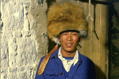
We detect and recognize the human faces in the video stream. Each face in the video is either recognized and the label is drawn next to their facial rectangle or it is labelled as unknown.

The video stream is obtained using Kinect v2 sensor. This sensor offers several data streams, we mention only the 2 relevant for our work:

  • RGB stream (resolution: 1920×1080, depth: 8bits)
  • Depth stream (resolution: 512×424, depth: 16bits)

The RGB stream is self-explanatory.  The depth stream consists of the values that denote the distance of the each pixel from the sensor.  The reliable distance lays between the 50 mms and extends to 8 meters. However, past the 4.5m mark, the reliability of the data is questionable. Kinect offers the methods that map the pixels from RGB stream to Depth stream and vice-versa.

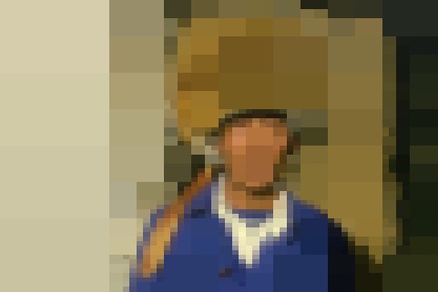
We utilize the facial data from RGB stream for the recognition. The depth data is used to enhance the face segmentation through the nose-tip detection.

First of all, the face recognizer has to be trained. The training is done only once. The state of the trained recognizer can be persisted in xml format and reloaded in the future without the need for repeated training. OpenCV offers implementation of three face recognition methods:

  • Eigenfaces
  • Fisherfaces
  • Local Binary Pattern Histograms

We used the Eigenfaces and Fisherfaces method. The code for creation of the face recognizer follows:

void initRecognizer()
{
	Ptr<FaceRecognizer> fr;
	fr = createEigenFaceRecognizer();
	trainRecognizer();
}

It is simple as that. Face recognizer that uses the Fisherfaces method can be created accordingly. The Ptr interface ensures the correct memory management.

All the faces presented to such recognizer would be labelled as unknown. The recognizer is not trained yet. The training requires the two vectors:

  • The vector of facial images in the OpenCV Mat format
  • The vector of integer values containing the identifiers for the facial images

These vectors can be created manually. This however is not sufficient for processing the large training sets. We thus provide the automated way to create these vectors. Data for each subject should be placed in a separate directory. Directories containing the subject data should be places within the single directory (referred to as root directory). The algorithm is given an access to the root directory. It processes all the subject directories and creates both the vector images and the vector labels. We think that the Windows API for accessing the file system is inconvenient. On the other hand, UNIX based systems offer convenient C API through the Dirent interface. Visual Studio compiler lacks the dirent interface. We thus used an external library to gain access to this convenient interface (http://softagalleria.net/dirent.php). Following code requires the library to run:

First we obtain the list of subject names. These stand for the directory names within the root directory. The subject names are stored in the vector of string values. It can be initialized manually or using the text file.

Then, for each subject, the path to their directory is created:

std::ostringstream fullSubjectPath;
fullSubjectPath << ROOT_DIRECTORY_PATH;
fullSubjectPath << "\\";
fullSubjectPath << subjectName;
fullSubjectPath << "\\";

We then obtain the list of file names that reside within the subject directory:

std::vector<std::string> DataProvider::getFileNamesForDirectory(const std::string subjectDirectoryPath)
{
	std::vector<std::string> fileNames;
	DIR *dir;
	struct dirent *ent;
	if ((dir = opendir(subjectDirectoryPath.c_str())) != NULL) {
		while ((ent = readdir(dir)) != NULL) {
			if ((strcmp(ent->d_name, ".") == 0) || (strcmp(ent->d_name, "..") == 0))
			{
				continue;
			}
			fileNames.push_back(ent->d_name);
		}
		closedir(dir);
	}
	else {
		std::cout << "Cannot open the directory: ";
		std::cout << subjectDirectoryPath;
	}
	return fileNames;
}

Then, the images are loaded and stored in vector:

std::vector<std::string> subjectFileNames = getFileNamesForDirectory(fullSubjectPath.str());

std::vector<cv::Mat> subjectImages;
for (std::string fileName : subjectFileNames)
{
	std::ostringstream fullFileNameBuilder;
	fullFileNameBuilder << fullSubjectPath.str();
	fullFileNameBuilder << fileName;
	cv::Mat subjectImage = cv::imread(fullFileNameBuilder.str());
		subjectImages.push_back(subjectImage);
}
return subjectImages;

In the end, label vector is created:

for (int i = 0; i < subjectImages.size(); i++){
	trainingLabels.push_back(label);
}

With images and labels vectors ready, the training is a one-liner:

fr->train(images,labels);

The recognizer is trained. What we need now is a video and depth stream to recognize from.
Kinect sensor is initialized by the following code:

void initKinect()
{
	HRESULT hr;

	hr = GetDefaultKinectSensor(&kinectSensor);
	if (FAILED(hr))
	{
		return;
	}

	if (kinectSensor)
	{
		// Initialize the Kinect and get the readers
		IColorFrameSource* colorFrameSource = NULL;
		IDepthFrameSource* depthFrameSource = NULL;

		hr = kinectSensor->Open();

		if (SUCCEEDED(hr))
		{
			hr = kinectSensor->get_ColorFrameSource(&colorFrameSource);
		}

		if (SUCCEEDED(hr))
		{
			hr = colorFrameSource->OpenReader(&colorFrameReader);
		}

		colorFrameSource->Release();

		if (SUCCEEDED(hr))
		{
			hr = kinectSensor->get_DepthFrameSource(&depthFrameSource);
		}

		if (SUCCEEDED(hr))
		{
			hr = depthFrameSource->OpenReader(&depthFrameReader);
		}

		depthFrameSource->Release();
	}

	if (!kinectSensor || FAILED(hr))
	{
		return;
	}
}

The following function obtains the next color frame from Kinect sensor:

Mat getNextColorFrame()
{
	IColorFrame* nextColorFrame = NULL;
	IFrameDescription* colorFrameDescription = NULL;
	ColorImageFormat colorImageFormat = ColorImageFormat_None;

	HRESULT errorCode = colorFrameReader->AcquireLatestFrame(&nextColorFrame);
	if (!SUCCEEDED(errorCode))
	{
		Mat empty;
		return empty;
	}

	if (SUCCEEDED(errorCode))
	{
		errorCode = nextColorFrame->get_FrameDescription(&colorFrameDescription);
	}
	int matrixWidth = 0;
	if (SUCCEEDED(errorCode))
	{
		errorCode = colorFrameDescription->get_Width(&matrixWidth);
	}
	int matrixHeight = 0;
	if (SUCCEEDED(errorCode))
	{
		errorCode = colorFrameDescription->get_Height(&matrixHeight);
	}
	if (SUCCEEDED(errorCode))
	{
		errorCode = nextColorFrame->get_RawColorImageFormat(&colorImageFormat);
	}
	UINT bufferSize;
	BYTE *buffer = NULL;
	if (SUCCEEDED(errorCode))
	{
		bufferSize = matrixWidth * matrixHeight * 4;
		buffer = new BYTE[bufferSize];
		errorCode = nextColorFrame->CopyConvertedFrameDataToArray(bufferSize, buffer, ColorImageFormat_Bgra);
	}
	Mat frameKinect;
	if (SUCCEEDED(errorCode))
	{
		frameKinect = Mat(matrixHeight, matrixWidth, CV_8UC4, buffer);
	}
	if (colorFrameDescription)
	{
		colorFrameDescription->Release();
	}
	if (nextColorFrame)
	{
		nextColorFrame->Release();
	}

	return frameKinect;
}

Analogous function obtains the next depth frame. The only change is the type and size of the buffer, as the depth frame is single channel 16 bit per pixel.
Finally, we are all set to do the recognition. The face recognition task consists of the following steps:

  1. Detect the faces in video frame
  2. Crop the faces and process them
  3. Predict the identity

For face detection, we use OpenCV CascadeClassifier. OpenCV provides the extracted features for the classifier for both the frontal and the profile faces. However, in video both the slight and major variations from these positions are present. We thus increase the tolerance for the false positives to prevent the cases when the track of the face is lost between the frames.
The classifier is simply initialized by loading the set of features using its load function.

CascadeClassifier cascadeClassifier;
cascadeClassifier.load(PATH_TO_FEATURES_XML);

The face detection is done as follows:

vector<Mat> getFaces(const Mat frame, vector<Rect_<int>> &rectangles)
{
	Mat grayFrame;
	cvtColor(frame, grayFrame, CV_BGR2GRAY);

	cascadeClassifier.detectMultiScale(grayFrame, rectangles, 1.1, 5);

	vector<Mat> faces;
	for (Rect_<int> face : rectangles){
		Mat detectedFace = grayFrame(face);
		Mat faceResized;
		resize(detectedFace, faceResized, Size(240, 240), 1.0, 1.0, INTER_CUBIC);
		faces.push_back(faceResized);
	}
	return faces;
}

With faces detected, we are set to proceed to recognition. The recognition process is as follows:

Mat colorFrame = getNextColorFrame();
vector<Rect_<int>> rectangles;
vector<Mat> faces = getFaces(colorFrameResized, rectangles);
int label = -1;
label = fr->predict(face);
string box_text = format("Prediction = %d", label);
putText(originalFrame, box_text, Point(rectangles[i].tl().x, rectangles[i].tl().y), FONT_HERSHEY_PLAIN, 1.0, CV_RGB(0, 255, 0), 2.0);

Nose tip detection is done as follows:

unsigned short minReliableDistance;
unsigned short maxReliableDistance;
Mat depthFrame = getNextDepthFrame(&minReliableDistance, &maxReliableDistance);
double scale = 255.0 / (maxReliableDistance - minReliableDistance);
depthFrame.convertTo(depthFrame, CV_16UC1, scale);

// detect nose tip
// only search for the nose tip in the head area
Mat deptHeadRegion = depthFrame(rectangles[i]);
			
// Nose is probably the local minima in the head area
double min, max;
Point minLoc, maxLoc;
minMaxLoc(deptHeadRegion, &min, &max, &minLoc, &maxLoc);
	minLoc.x += rectangles[i].x;
	minLoc.y += rectangles[i].y;

// Draw the circle at proposed nose position.
circle(depthFrame, minLoc, 5, 255, -1);

To conclude, we provide a simple implementation that allows the detection and recognition of human faces within a video. The room for improvement is that rather than allowing more false positives in detection phase, the detected nose tip can be used for face tracking.

Posted on

Medical image segmentation

Martin Tamajka

In this project, our goal was to apply image segmentation techniques to dense volume of standard medical data.

Oversegmentation

Our method is based on oversegmentation to supervoxels (similar to superpixels, but in 3D volume). Such oversegmentation dramatically decreases processing time and has many other advantages over working directly with voxels. Oversegmentation is done using SLIC algorithm (http://www.kev-smith.com/papers/SLIC_Superpixels.pdf). Implementation that we use was created by authors and does not depend on any other library. This comes at cost of necessity to transform images in OpenCV format to C++ arrays. SLIC allows to choose between supervoxel compactness (or regularity of shape) and intensity homogeneity. In our work, we decided to prefer homogeneity over regularity, because different tissues in anatomical organs have their typical intensities.

tamajka_oversegmentation
Oversegmented MRI slice – it can be seen that supervoxels adhere boundaries.

Merging supervoxels


After we oversegmented images, we created object representation of volume. Our object representation (SLIC3D) has following attributes:

vector&amp;amp;lt;Supervoxel*&amp;amp;gt;				m_supervoxels;
std::unordered_map&amp;amp;lt;int, Supervoxel*&amp;amp;gt;	m_supervoxelsMap;
int	m_height;
int	m_width;
int	m_depth;

The most important is the vector of Supervoxel pointers. Supervoxel is our basic class providing important information about contained voxels, can generate features that can be used in classification process and (very important) knows its neighbouring supervoxels. Currently, Supervoxel can generate 3 kinds of features:

float Supervoxel::AverageIntensity()
{
	return m_centroid-&amp;amp;gt;intensity;
}

float Supervoxel::AverageQuantileIntensity(float quantile)
{
	assert(quantile &amp;amp;gt;= 0 &amp;amp;amp;&amp;amp;amp; quantile &amp;amp;lt;= 1);

	float intens = 0;

	int terminationIndex = quantile * m_points.size();
	for (int i = 0; i &amp;amp;lt; terminationIndex; i++)
		intens += m_points[i]-&amp;amp;gt;intensity;

	return intens / terminationIndex;
}

float Supervoxel::MedianIntensity()
{
	return m_points[m_points.size() / 2]-&amp;amp;gt;intensity;
} 

SLIC3D class (the one containing supervoxels) has method where “all magic happens” - MergeSimilarSupervoxels. As stated in its name, method merges voxels. Method performs given number of iterations. In each iteration, method takes random supervoxels, compares it with its neighbours and if a neighbour and examined supervoxels have similar average intensity, the latter one is merged to the examined one. Code can be seen right below.

bool SLIC3D::MergeSimilarSupervoxels()
{
	vector&amp;amp;lt;Supervoxel*&amp;amp;gt; supervoxelsToBeErased;
	for (int i = 0; i &amp;amp;lt; 10000; i++)
	{
		cout &amp;amp;lt;&amp;amp;lt; i &amp;amp;lt;&amp;amp;lt; " " &amp;amp;lt;&amp;amp;lt; m_supervoxels.size() &amp;amp;lt;&amp;amp;lt; endl;
		std::sort(m_supervoxels.begin(), m_supervoxels.end(), helper_sortFunctionByAvgIntensity);
		
		Supervoxel* brightestSupervoxel = m_supervoxels[rand() % (m_supervoxels.size() - 1)];
		std::unordered_map&amp;amp;lt;int, Supervoxel*&amp;amp;gt; nb = *(brightestSupervoxel-&amp;amp;gt;GetNeighbours());

		int numberOfIterations = 0;
		vector&amp;amp;lt;int&amp;amp;gt; labelsToBeErased;
		for (auto it = nb.begin(); it != nb.end(); it++)
		{
			if (std::min(brightestSupervoxel-&amp;amp;gt;AverageIntensity(), it-&amp;amp;gt;second-&amp;amp;gt;AverageIntensity()) / std::max(brightestSupervoxel-&amp;amp;gt;AverageIntensity(), it-&amp;amp;gt;second-&amp;amp;gt;AverageIntensity()) &amp;amp;gt; 0.95)
			{
				helper_mergeSupervoxels(brightestSupervoxel, it-&amp;amp;gt;second);
				labelsToBeErased.push_back(it-&amp;amp;gt;second-&amp;amp;gt;GetLabel());
				supervoxelsToBeErased.push_back(it-&amp;amp;gt;second);
			}
			else
			{
				//cout &amp;amp;lt;&amp;amp;lt; "nope" &amp;amp;lt;&amp;amp;lt; endl;
			}
			numberOfIterations++;
		}

		for (int i = 0; i &amp;amp;lt; labelsToBeErased.size(); i++)
		{
			Supervoxel* toBeRemoved = m_supervoxelsMap[labelsToBeErased[i]];

			if (NULL == toBeRemoved)
				continue;

			std::unordered_map&amp;amp;lt;int, Supervoxel*&amp;amp;gt; nbb = *(toBeRemoved-&amp;amp;gt;GetNeighbours());

			for (auto it = nbb.begin(); it != nbb.end(); it++)
			{
				try
				{
					it-&amp;amp;gt;second-&amp;amp;gt;AddNeighbour(brightestSupervoxel);
					it-&amp;amp;gt;second-&amp;amp;gt;RemoveNeighbour(toBeRemoved);
					brightestSupervoxel-&amp;amp;gt;AddNeighbour(it-&amp;amp;gt;second);
				}
				catch (Exception e)
				{
					cout &amp;amp;lt;&amp;amp;lt; "exc: " &amp;amp;lt;&amp;amp;lt; e.msg &amp;amp;lt;&amp;amp;lt; endl;
				}
			}
		}
		
		for (int i = 0; i &amp;amp;lt; labelsToBeErased.size(); i++)
		{
			Supervoxel* toBeRemoved = m_supervoxelsMap[labelsToBeErased[i]];
			m_supervoxelsMap.erase(labelsToBeErased[i]);
			//delete toBeRemoved; //COMMENT
		}

		brightestSupervoxel-&amp;amp;gt;RecalculateCentroid();

		m_supervoxels.clear();
		for (auto it = m_supervoxelsMap.begin(); it != m_supervoxelsMap.end(); ++it)
		{
			m_supervoxels.push_back(it-&amp;amp;gt;second);
		}
	}

	for (int i = 0; i &amp;amp;lt; supervoxelsToBeErased.size(); i++)
		;// delete supervoxelsToBeErased[i];	//COMMENT - to be considered if delete

	return true;
} 

Results of merging in such form highly depend on chosen similarity level. In the picture below left we can see result of applying similarity level 0.95. In the image right the value of similarity level was chosen to be 0.65.

tamajka_results

We also tried to train SVM to classify brain and non-brain structures using just these features. We got 4 successful classifications of 5. With classification we will continue later.

Posted on

Lane markers detection

Michal Polko

In this project, we detect lane markers in videos taken with dashboard camera.

Process

  1. Convert a video frame to grayscale, boost contrast and apply dilation operator to highlight lane markers in the frame.
    polko_highlighted_markers
    Highlighted lane markers.
    cvtColor(frame, frame_bw, CV_RGB2GRAY);
    frame_bw.convertTo(frame_bw, CV_32F, 1.0 / 255.0);
    pow(frame_bw, 3.0, frame_bw);
    frame_bw *= 3.0;
    frame_bw.convertTo(frame_bw, CV_8U, 255.0);
    dilate(frame_bw, frame_bw, getStructuringElement(CV_SHAPE_RECT, Size(3, 3)));
    
  2. Apply the Canny edge detection to find edges.
    polko_edges
    Application of the Canny edge detection.
    int cny_threshold = 100;
    Canny(frame_bw, frame_edges, cny_threshold, cny_threshold * 3, 3);
    
  3. Apply the Hough transform to find line segments.
    vector<Vec4i> hg_lines;
    HoughLinesP(frame_edges, hg_lines, 1, CV_PI / 180, 15, 15, 2);
    
  4. Since the Hough transform returns all line segments, not only those around lane markers, it is necessary to filter the results.
    1. We create two lines that describe boundaries of the current lane (hypothesis).
      1. We place two converging lines in the frame.
      2. Using brute-force search, we try to find position where they capture as many line segments as possible.
      3. Since road in the frame can have more than one lane, we try to find result as narrow as possible.
    2. We select line segments that are captured by the created hypothesis, mark them as lane markers and draw them.
    3. Each frame, we take the detected lane markers from the previous frame and perform linear regression to adjust the hypothesis (continuous adjustment).
    4. If we cannot find lane markers in more than 5 successive frames (due to failure of continuous adjustment, lane change, intersection, …), we create a new hypothesis.
    5. If the hypothesis is too wide (almost full width of the frame), we create a new one, because arrangement of road lanes might have changed (e.g. additional lane on freeway).
  5. To distinguish between solid and dashed lane markers, we calculate coverage of the hypothesis by line segments. If the coverage is less than 60%, it is a dashed line; if more, it is a solid line.

    polko_result
    Filtered result of the Hough transform + detection of solid/dashed lines.
Posted on

Split and merge

Matus Pikuliak

In our work we have implemented segmentation algorithm split-and-merge. We have designed each step of this algorithm processing original image into segmented image composed of homogeneous regions. We have used OpenCV library to build our solution.

Our method has 4 steps. We will demonstrate their effect on image depicted in Figure 1.

pikuliak_original
Original photo
  1. Pre-processing
    First we convert image from RGB color space to Lab. Then we blur the image to remove various blemishes, that could potentially halt the splitting phase

    cv::cvtColor(image, image, CV_BGR2Lab);
    cv::GaussianBlur(image, image, Size(5,5), 0, 0);
    
  2. Splitting
    In splitting phase we divide image to same-sized quarters. We compute the standard deviation of each of the dimensions of color space. If these values for given quarter exceed adjustable thresholds, we recursively divide this quarter as well. This go on, until the created quarters are big enough. If they one of their dimensions is smaller than what we have set as minimum length (9), dividing is stopped.
    If the values of deviations does not exceed thresholds, dividing is stopped and given quarter is completely filled with its mean color. Examples of splitting can be seen on Figure 2.

    pikuliak_splitting
    After splitting.
    void split(roi) {
    	if (roi.standard_deviation > threshold) {
    		quarters = roi.get_quarters
    			quarters.each{
    			split(quarter)
    		}
    	}
    	else {
    		roi.paint
    	}
    }
    
  3. Merging
    Split image is subsequently processed with merge operation. This operation merges neighboring regions with similar features. In our work we use only the dimensions of Lab color space and therefor we are merging regions with similar color. The similarity is again calculated using thresholds for individual dimensions of color space. Result of this operation can be seen on Figure 3. We can see that a lot of rectangular regions were merged into bigger super-regions. This effect can be seen on every part of the image.

    pikuliak_merging
    After merging.
    // runs floodFill for every unaffected ROI
    void merge() {
    	imageorg = image.clone();
    	for (std::list<list_item>::iterator it = rois.begin(); it != rois.end(); it++) {
    		Vec3b c = image.at<Vec3b>(it->point);
    		Vec3b c2 = imageorg.at<Vec3b>(it->point);
    		if (c[0] == c2[0] && c[1] == c2[1] && c[2] == c2[2]) {
    			floodFill(image, it->point, Scalar(c[0], c[1], c[2]), 0,
    				Scalar(l_treshold, ab_treshold, ab_treshold),
    				Scalar(l_treshold, ab_treshold, ab_treshold));
    		}
    	}
    }
    
  4. Post-processing
    As we can see there are some artifacts left, mainly on the edges of different bigger regions. These artifacts are result of splitting, which can not handle parts of images, where there are sudden changes from one dominant color to other. In order to remove these artifacts and improve overall we are using several morphological operations followed with yet another merging of color regions. Result of post-processing can be seen on Figure 4, which is at the same time final result of our method for this image.

    pikuliak_final
    Final image.
    Mat kernel = getStructuringElement(MORPH_ELLIPSE,Size(Morph, Morph));
    dilate(image, image, kernel,Point(-1,-1),2);
    erode(image, image, kernel,Point(-1,-1),2);
    erode(image, image, kernel,Point(-1,-1),2);
    dilate(image, image, kernel,Point(-1,-1),2);
    

Settings

There are several settings that can affect the result of our method:

  • color dimensions – we can change how much is our method sensitive to changes in individual dimensions of our color space. Higher sensitivity leads to smaller regions after split phase and worse merging. Lower sensitivity can on the other hand lead to results which are too rough.
  • minimum size of region – this setting can affect resulting granularity of final image. Too small minimum regions lead to over-split image, while too large lead to inaccurate results.
  • color space – color space is another setting that can change the outcome of our method. In our experiments we find out, that the Lab color space outperforms RGB color space in generality. Lab was providing satisfactory results to almost all of our testing images with similar settings. RGB on the other hand requires more tweaking for optimal results.

Conclusion

We have successfully implemented split-and-merge segmentation algorithm and tested in on variety of images with different features and characteristics. We conclude that our implemented method is fast and reliable.

Posted on

Free parking spots detection

Jan Onder

The goal of this project is to determine the state of a parking lot, more precisely the number of parking spaces. Basically this project is divided to two interconnected parts. One to determine number of parking spots from image, for example from first frame of video from camera, monitoring the parking lot, and second to determine wheter, or not is there a movement on the parking lot.

The process:

  1. We get parking lines from image of parking lot and get rid of noise:
    Canny(inputImage, helpMatrix, 450, 400, 3);
    cvtColor(helpMatrix, helpMatrix2, CV_GRAY2BGR);
    vector<Vec4i> lines;
    HoughLinesP(helpMatrix, lines, 1, CV_PI / 180, 7, 10, 10);
    for (size_t i = 0; i < lines.size(); i++)
    {
    	Vec4i l = lines[i];
    	line(helpMatrix2, Point(l[0], l[1]), Point(l[2], l[3]), Scalar(0, 0, 255), 5, CV_AA)
    }
    Mat element2 = getStructuringElement(CV_SHAPE_RECT, Size(3, 3));
    cv::erode(helpMatrix2, helpMatrix2, element);
    cv::dilate(helpMatrix2, helpMatrix2, element2);
    

    onder_edges
    Original Image (A), Canny edges with noise (B), HoughLines without noise (C)
  2. We use double dilate and substract their results to get mask of lines:
    morphologyEx(helpMatrix2, mark, CV_MOP_DILATE, element,Point(-1,-1), 3);
    morphologyEx(helpMatrix2, mark2, CV_MOP_DILATE, element, Point(-1, -1), 2);
    result = mark - mark2;
    

    onder_mask
    Result of dilating and substracting
  3. We use Canny and Hough lines, this time for removing the connecting line between each parking spot:
    Canny(resu, mark, 750, 800, 3);
    cvtColor(mark, mark2, CV_GRAY2BGR);
    mark2 = Scalar::all(0);
    vector<Vec4i> lines3;
    HoughLinesP(mark, lines3, 1, CV_PI / 180, 20, 15, 10);
    for (size_t i = 0; i < lines3.size(); i++)
    {
    	Vec4i l = lines3[i];
    	line(mark2, Point(l[0], l[1]), Point(l[2], l[3]), Scalar(0, 0, 255), 2, CV_AA);
    }
    

    onder_connection
    Result of Hough lines to remove connection between lines in mask
  4. We use this as a mask for finding contours for the Watershed algorithm and get result with detected parking spots, each colored with different color:
    vector<vector<Point> > contours;
    vector<Vec4i> hierarchy;
    findContours(markerMask, contours, hierarchy, RETR_CCOMP, CHAIN_APPROX_SIMPLE);
    int contourID = 0;
    for (; contourID >= 0; contourID = hierarchy[contourID][0], parkingSpaceCount++)
    {
    	drawContours(markers, contours, contourID, Scalar::all(parkingSpaceCount + 1), -1, 8, hierarchy, INT_MAX);
    }
    watershed(helpMatrix2, markers);
    Mat wshed(markers.size(), CV_8UC3);
    for (i = 0; i < markers.rows; i++)
    	for (j = 0; j < markers.cols; j++)
    	{
    		int index = markers.at<int>(i, j);
    		if (index == -1)
    			wshed.at<Vec3b>(i, j) = Vec3b(255, 255, 255);
    		else if (index <= 0 || index > parkingSpaceCount)
    			wshed.at<Vec3b>(i, j) = Vec3b(0, 0, 0);
    		else
    			wshed.at<Vec3b>(i, j) = colorTab[index - 1];
    	}
    

    onder_watershed
    Result of watershed algorithm with detected parking spots
  5. If our user is not satisfied with this result, he can always draw the seeds for watershed himself, or just adjust these seeds (img is the name of matrix, where user can see markers and markerMask matrix, where seeds are stored):
    Point prevPt(-1, -1);
    static void onMouse(int event, int x, int y, int flags, void*)
    {
    	if (event == EVENT_LBUTTONDOWN) prevPt = Point(x, y);
    	else if (event == EVENT_MOUSEMOVE && (flags & EVENT_FLAG_LBUTTON))
    	{
    		Point pt(x, y);
    		if (prevPt.x < 0)
    			prevPt = pt;
    		line(markerMask, prevPt, pt, Scalar::all(255), 5, 8, 0);
    		line(img, prevPt, pt, Scalar::all(255), 5, 8, 0);
    		prevPt = pt;
    		imshow("image", img);
    	}
    }
    

    onder_input_seeds
    User inputing seeds for watershed algorithm
  6. We have our spots stored, so we know their exact location, now its time to determine, wheter, or not check the lot again, if some vehicles are moving. For this purpose we need to detect movement on the lot with backgroundSubstraction, which can constantly learn what is static in image:
    Ptr<BackgroundSubtractor> pMOG2;
    pMOG2 = new BackgroundSubtractorMOG2(3000, 20.7,true);
    
  7. We will give the MOG every frame captured from video feed and see what it results:
    pMOG2->operator()(frame, matMaskMog2,0.0035);
    imshow("MOG2", matMaskMog2);
    

    onder_MOG
    Result of MOG substraction
  8. As we can see, there is some noise detected – this noise represents for example moving leaves on trees, so it is necessary to remove it:
    cv::morphologyEx(matMaskMog2, matMaskMog2, CV_MOP_ERODE, element);
    cv::medianBlur(matMaskMog2, matMaskMog2, 3);
    cv::morphologyEx(matMaskMog2, matMaskMog2, CV_MOP_DILATE, element2);
    
  9. Finally we find coordinates of moving object from MOG and draw a rectangle with random color around it (result can be seen at the top):
    scv::findContours(matMaskMog2, contours, CV_RETR_EXTERNAL, CV_CHAIN_APPROX_NONE);
    vector<vector<Point> > contours_poly(contours.size());
    vector<Rect> boundRect(contours.size());
    
    for (int i = 0; i < contours.size(); i++)
    {
    approxPolyDP(Mat(contours[i]), contours_poly[i], 3, true);
    	boundRect[i] = boundingRect(Mat(contours_poly[i]));		
    }
    RNG rng(01);
    for (int i = 0; i< contours.size(); i++)
    {
    Scalar color = Scalar(rng.uniform(0, 255), rng.uniform(0, 255), rng.uniform(0, 255)); 
    	rectangle(frame, boundRect[i].tl(), boundRect[i].br(), color, 2, 8, 0);
    }
    

Result:

We have a functional parking spot detection, which means we can easily determine how much parking spots our parking lot have. We also have stored where are these parking spots exactly located. From the camera feed, we can detect car movement and also determine, on which coordinates the movement stopped. We did not implemented the function to connect these infomormation sources, but it can be easily added.

Limitations:

  • For parking spots detection we need an empty lot. Otherwise it will be nearly impossible to determine where are these spots exactly located, mainly if vehicles are not parking at their exact center.
  • For movement detection, we need static camera feed, becouse of used MOG method, which constantly learns what is background and which object are moving.
  • Parking spots detection is not perfect, it still needs some user correction to determine exact number of parking spots.
Posted on

Panorama – Image registration

Vladimir Ogurcak

The main objective of this project is to create panoramic image from sequence of two or more overlapping images using OpenCV. We assume then overlap of two adjacent images is more than 30%, vertical variation of all images is minimal and images are ordered from left to right.

The main idea of this algorithm is based on independent image stitching of two adjacent images and recurrent stitching of results until complete panorama image isn’t created. The code below shows this idea:

AutomaticPanorama(vector<Mat> results){			//results contains all input images
	vector<Mat> partialResults = vector<Mat>();
	while (results.size() != 1){
		//Stitch all adjacent images and save result as partial result
		for (int i = 0; i < results.size() - 1; i++){
			Mat panoramaResult = Panorama(results[i], results[i + 1]);
			partialResults.push_back(panoramaResult);
		}
		//results = paritalResults
		vector<Mat> temp = results;
		results = partialResults;
		partialResults = temp;
		partialResults.clear();
	}
}

Function Panorama(results[i], results[i + 1]) is custom implementation of image stitching. This function uses local detector and descriptor SIFT, Brute-force keypoint matcher and perspective transformation to realize image registration and stitching. Individual steps (parts) of function are described below. In this project we also tried to use other detectors like SURF, ORB and descriptors like SURF, ORB, BRISK and FREAK, but SIFT and SURF appears to be the best choices.

OpenCV functions

SiftFeatureDetector, SiftDescriptorExtractor, BFMatcher, drawMatches, findHomography, perspectiveTransform, warpPerspective, imshow, imwrite

Input

ogurcak_input
Left and right image.

Panorama

  1. Calculate keypoints for left and right image using SIFT feature detector:
    SiftFeatureDetector detector = SiftFeatureDetector();
    vector<KeyPoint> keypointsPrev, keypointsNext;
    detector.detect(imageNextGray, keypointsNext);
    detector.detect(imagePrevGray, keypointsPrev);
    

    ogurcak_keypoints
    Left and right image with keypoints.
  2. Calculate local descriptor for all keypoints using SIFT descriptor:
    SiftDescriptorExtractor extractor = SiftDescriptorExtractor();
    Mat descriptorsPrev, descriptorsNext;
    extractor.compute(imageNextGray, keypointsNext, descriptorsNext);
    extractor.compute(imagePrevGray, keypointsPrev, descriptorsPrev);
    
  3. For keypoint descriptors from left image find corresponding keypoint descriptors in right image using Brute-Force matcher:
    BFMatcher bfMatcher;
    bfMatcher.match(descriptorsPrev, descriptorsNext, matches);
    

    ogurcak_keypoint_pairs
    Pairs of key points (every fifth match)
  4. Find only good matches. Good matches are pairs of keypoints which vertical coordinate variation is less than 5%:
    vector<DMatch> goodMatches;
    int minDistance = imagePrevGray.rows / 100 * VERTICALVARIATION;
    goodMatches = FindGoodMatches(matches, keypointsPrev, keypointsNext, minDistance);
    

    ogurcak_good_pairs
    Good matches (5% variation)
  5. Find homography matrix for perspective transformation of right image. Use only good keypoints for computing homography matrix:
    Mat homographyMatrix;
    homographyMatrix = findHomography(pointsNext, pointsPrev, CV_RANSAC);
    
  6. Warp right image using homography matrix from previous step:
    Mat warpImageNextGray;
    warpPerspective(imageNextGray, warpImageNextGray, homograpyMatrix, Size(imageNextGray.cols + imagePrevGray.cols, imageNextGray.rows));
    

    ogurcak_warp
    Warped right image
  7. Calculate left image and right (warped) image corners:
    vector<Point2f> cornersPrev, cornersNext;
    SetCorners(imagePrevGray, imageNextGray, &cornersPrev, &cornersNext, homograpyMatrix);
    

    ogurcak_corners
    Left (blue) and right (green) image boundaries
  8. Find overlap coordinates of left and right images:
    int overlapFromX, overlapToX;
    if (cornersNext[0].x < cornersNext[3].x){
    	overlapFromX = cornersNext[0].x;
    }
    else{
    	overlapFromX = cornersNext[3].x;
    }
    overlapToX = cornersPrev[1].x;
    
  9. Join left and right (warped) image using linear interpolation in overlapped area. Both images contributes with 100% of its pixels outside the overlapping area. Left image contribute with 100% at the beginning of overlapping area and gradually decreases its contribution to 0% at the end. Right image contribute opposite way from 0% at beginning to 100 % at the end:
    Mat result = Mat::zeros(warpImageNextGray.rows, warpImageNextGray.cols, CV_8UC3);
    DrawTransparentImage(imagePrevGray, cornersPrev, warpImageNextGray, cornersNext, &result, overlapFromX, overlapToX);
    
  10. Crop joined image:
    Rect rectrangle(0, 0, cornersNext[1].x, result.rows);
    result = result(rectrangle);
    

Limitation

  • Sufficient overlap of adjavent images. We assume more than 30%.
  • Maximum number of input images is generally less or equals to 5. The deformation of perspective transformation causes failure of algorithm in larger set of input images.
  • Input images has to be sorted for example from left to right.
  • Panorama of distance objects gives better results than panorama of nearby objects.

Results

ogurcak_goldongate
Goldangate bridge – Panorama of 5 images
ogurcak_mountains
Mountains – Panorama of 5 images

ogurcak_shanghai
Shanghai – Panorama of 5 images


Comparison of different keypoint detectors and descriptors

Detector / Descriptor Number of all matches Number of good matches Result
SIFT / SIFT 3064 976 Successful
SURF / SURF 3217 1309 Successful
ORB / ORB 3000 1113 Successful
SIFT / BRIEF 2827 790 Successful
SIFT / BRISK 1012 128 Failure
SIFT / FREAK 1154 151 Failure
Posted on

Motion analysis in CCTV records

Filip Mazan

This project deals with analysis of video captures from CCTVs to detect people’s motion and extract their trajectories in time. The output of this project is a relatively short video file containing only frames of the original where the movement was detected along with shown trajectories of people. The second output consists of cumulative image of all trajectories. This can be later used to classify trajectories as (not) suspicious.

  1. Each frame of input video is converted into grayscale and median filtered to remove noise
  2. First 30 seconds of video is used as a learning phase for MOG2 background subtractor
  3. For each next frame the MOG2 mask is calculated and morphological closing is applied to it
  4. If count of non-zero pixels is greater than a set threshold, we claim there is a movement present
    1. Good features to track are found if there is not many left
    2. Optical flow is calculated
    3. Each point which has moved is stored along with frame number
  5. If there is no movement on current frame, postprocess last movement interval (if any)
    1. All stored tracking points (x, y, frame number) from previous phase are clusterized by k-means into variable number of centroids
      mazan_tracking_points
    2. All centroids are sorted by their frame number dimension
    3. Trajectory is drawn onto the output frame
      mazan_single_trajectory
    4. Movement sequence is written into the output video file along with continuously drawn trajectory

Following image shows the sum of all trajectories found in 2 hours long input video. This can be used to classify trajectories as (not) suspicious.

mazan_all_trajectories