Vladimir Ogurcak
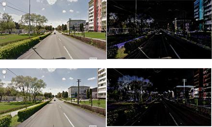
The main objective of this project is to create panoramic image from sequence of two or more overlapping images using OpenCV. We assume then overlap of two adjacent images is more than 30%, vertical variation of all images is minimal and images are ordered from left to right.
The main idea of this algorithm is based on independent image stitching of two adjacent images and recurrent stitching of results until complete panorama image isn’t created. The code below shows this idea:
AutomaticPanorama(vector<Mat> results){			//results contains all input images
	vector<Mat> partialResults = vector<Mat>();
	while (results.size() != 1){
		//Stitch all adjacent images and save result as partial result
		for (int i = 0; i < results.size() - 1; i++){
			Mat panoramaResult = Panorama(results[i], results[i + 1]);
			partialResults.push_back(panoramaResult);
		}
		//results = paritalResults
		vector<Mat> temp = results;
		results = partialResults;
		partialResults = temp;
		partialResults.clear();
	}
}
Function Panorama(results[i], results[i + 1]) is custom implementation of image stitching. This function uses local detector and descriptor SIFT, Brute-force keypoint matcher and perspective transformation to realize image registration and stitching. Individual steps (parts) of function are described below. In this project we also tried to use other detectors like SURF, ORB and descriptors like SURF, ORB, BRISK and FREAK, but SIFT and SURF appears to be the best choices.
OpenCV functions
SiftFeatureDetector, SiftDescriptorExtractor, BFMatcher, drawMatches, findHomography, perspectiveTransform, warpPerspective, imshow, imwrite
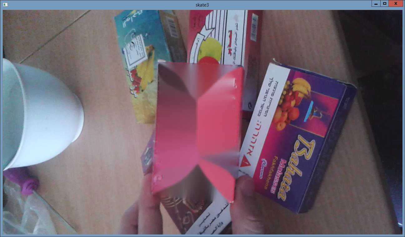
Input
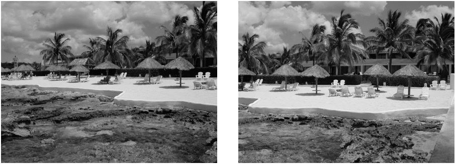
Panorama
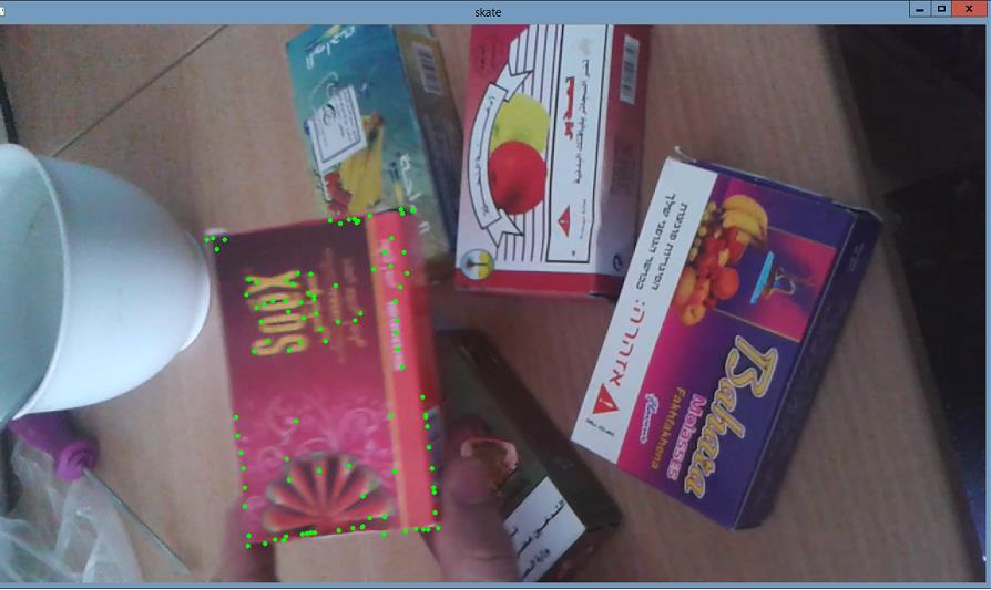
- Calculate keypoints for left and right image using SIFT feature detector:
SiftFeatureDetector detector = SiftFeatureDetector();
vector<KeyPoint> keypointsPrev, keypointsNext;
detector.detect(imageNextGray, keypointsNext);
detector.detect(imagePrevGray, keypointsPrev);
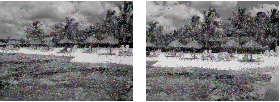
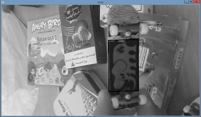
Left and right image with keypoints. - Calculate local descriptor for all keypoints using SIFT descriptor:
SiftDescriptorExtractor extractor = SiftDescriptorExtractor();
Mat descriptorsPrev, descriptorsNext;
extractor.compute(imageNextGray, keypointsNext, descriptorsNext);
extractor.compute(imagePrevGray, keypointsPrev, descriptorsPrev);
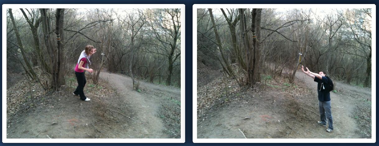
- For keypoint descriptors from left image find corresponding keypoint descriptors in right image using Brute-Force matcher:
BFMatcher bfMatcher;
bfMatcher.match(descriptorsPrev, descriptorsNext, matches);
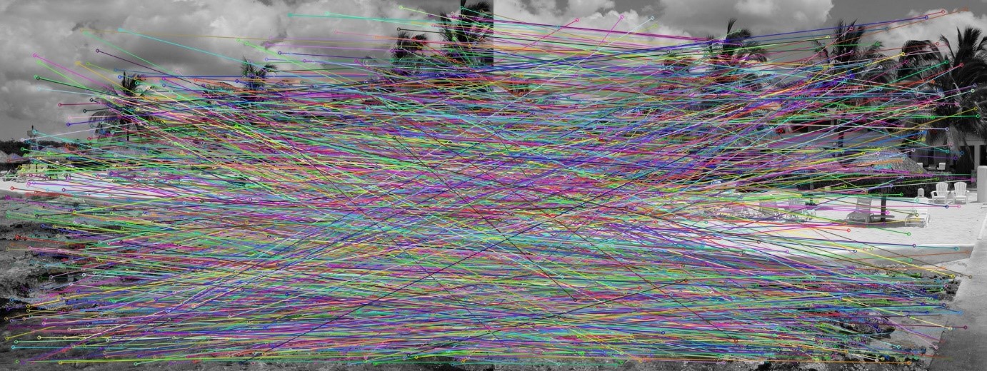
Pairs of key points (every fifth match) - Find only good matches. Good matches are pairs of keypoints which vertical coordinate variation is less than 5%:
vector<DMatch> goodMatches;
int minDistance = imagePrevGray.rows / 100 * VERTICALVARIATION;
goodMatches = FindGoodMatches(matches, keypointsPrev, keypointsNext, minDistance);
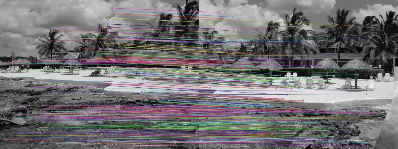
Good matches (5% variation) - Find homography matrix for perspective transformation of right image. Use only good keypoints for computing homography matrix:
Mat homographyMatrix;
homographyMatrix = findHomography(pointsNext, pointsPrev, CV_RANSAC);
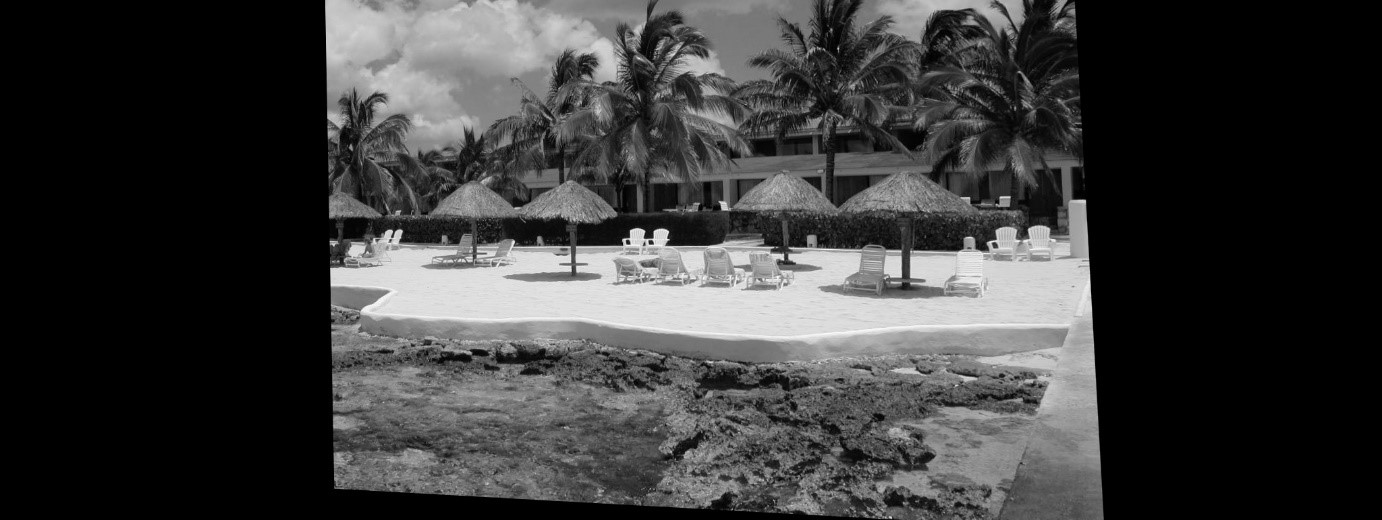
- Warp right image using homography matrix from previous step:
Mat warpImageNextGray;
warpPerspective(imageNextGray, warpImageNextGray, homograpyMatrix, Size(imageNextGray.cols + imagePrevGray.cols, imageNextGray.rows));

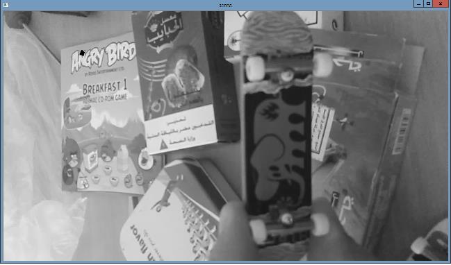
Warped right image - Calculate left image and right (warped) image corners:
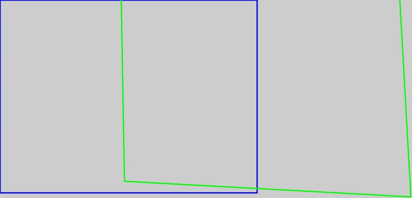
vector<Point2f> cornersPrev, cornersNext;
SetCorners(imagePrevGray, imageNextGray, &cornersPrev, &cornersNext, homograpyMatrix);
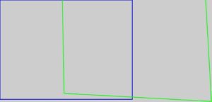
Left (blue) and right (green) image boundaries - Find overlap coordinates of left and right images:
int overlapFromX, overlapToX; if (cornersNext[0].x < cornersNext[3].x){ overlapFromX = cornersNext[0].x; } else{ overlapFromX = cornersNext[3].x; } overlapToX = cornersPrev[1].x; - Join left and right (warped) image using linear interpolation in overlapped area. Both images contributes with 100% of its pixels outside the overlapping area. Left image contribute with 100% at the beginning of overlapping area and gradually decreases its contribution to 0% at the end. Right image contribute opposite way from 0% at beginning to 100 % at the end:
Mat result = Mat::zeros(warpImageNextGray.rows, warpImageNextGray.cols, CV_8UC3);
DrawTransparentImage(imagePrevGray, cornersPrev, warpImageNextGray, cornersNext, &result, overlapFromX, overlapToX);
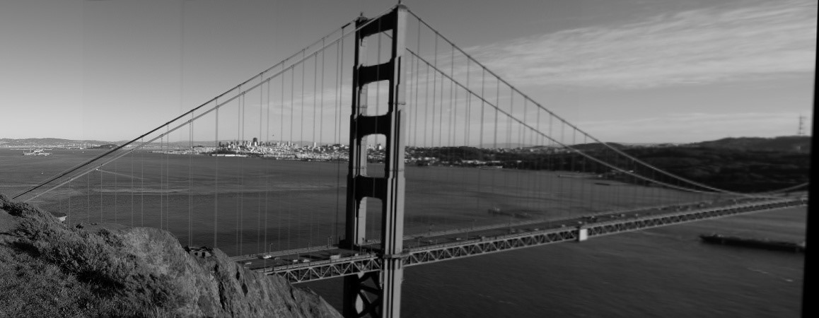
- Crop joined image:
Rect rectrangle(0, 0, cornersNext[1].x, result.rows);
result = result(rectrangle);
Limitation
- Sufficient overlap of adjavent images. We assume more than 30%.
- Maximum number of input images is generally less or equals to 5. The deformation of perspective transformation causes failure of algorithm in larger set of input images.
- Input images has to be sorted for example from left to right.
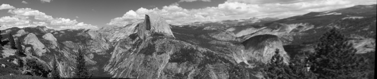
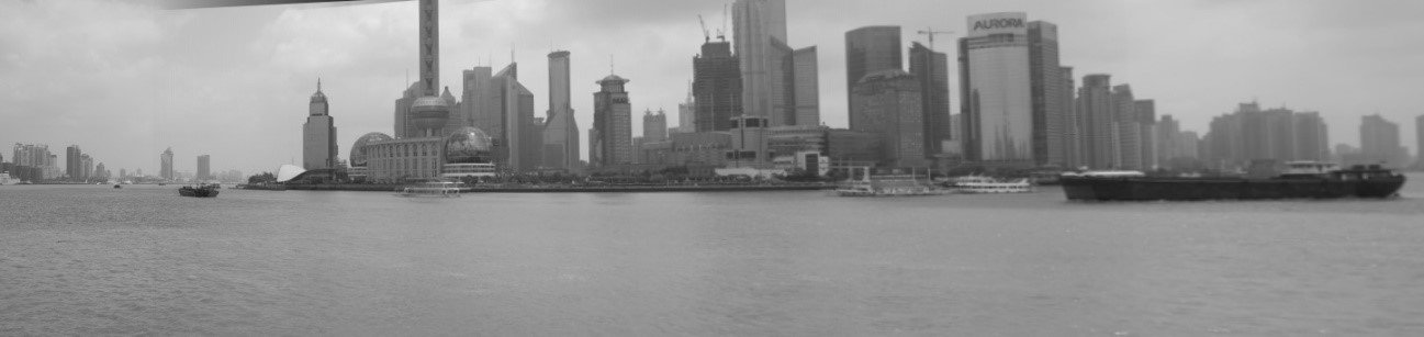
- Panorama of distance objects gives better results than panorama of nearby objects.
Results
Comparison of different keypoint detectors and descriptors
| Detector / Descriptor | Number of all matches | Number of good matches | Result |
|---|---|---|---|
| SIFT / SIFT | 3064 | 976 | Successful |
| SURF / SURF | 3217 | 1309 | Successful |
| ORB / ORB | 3000 | 1113 | Successful |
| SIFT / BRIEF | 2827 | 790 | Successful |
| SIFT / BRISK | 1012 | 128 | Failure |
| SIFT / FREAK | 1154 | 151 | Failure |