Posted on

Visual Finger Counter

Gabriela Brndiarova

Aim of this project was implementing of finger counter with OpenCV. Input from ordinary webcam was used and it is possible to get realtime results, now. At first, we segmented hand using camshift algorithm. After that, we got hand contours and convexity defect. There was used very simple algorithm to count fingers when the convexity defects were known.

Function used: calcHist, calcBackProject, CamShift, threshold, morphologyEx, findContours, convexHull, convexityDefects

Input

brndiarova_input

The process

  1. Selecting a litle square on the hand with the mouse.
  2. Calculating histogram from selected range.
    Mat frame, hsv, hue, mask, hist = Mat::zeros(200, 320, CV_8UC3);
    inRange(hsv, Scalar(0, smin, 10), Scalar(180, 256, 256), mask); 
    hue.create(hsv.size(), hsv.depth());
    mixChannels(&hsv, 1, &hue, 1, ch, 1);
    Mat roi(hue, selection), maskroi(mask, selection);
    calcHist(&roi, 1, 0, maskroi, hist, 1, &hsize, &phranges);
    
  3. Getting back projection of image.
    calcBackProject(&hue, 1, 0, hist, backproj, &phranges);
    
  4. Camshift application to get selection of hand.
    CamShift(backproj, trackWindow, TermCriteria( CV_TERMCRIT_EPS | V_TERMCRIT_ITER, 10, 1 ));
    
  5. Manual making the selection bigger (it is important to have whole fingers in the selection), but not too big because of face. If face is in the selection, hand segmentation is no longer possible.
  6. The selection of hand is cut off and rotate to natural position for human (fingers point to the top).
    int angle = trackBox.angle;
    Size rect_size = trackBox.size;
    if (angle >90){
    	angle -= 180;
    	angle *= -1;
    }
    M = getRotationMatrix2D(trackBox.center, angle, 1.0);
    warpAffine(backprojMask, rotatedMask, M, backprojMask.size(), INTER_CUBIC);
    getRectSubPix(rotatedMask, rect_size, trackBox.center, croppedMask);
    
  7. Treshold application.
    threshold(croppedMask, croppedMask, tresholdValue, 255 , THRESH_BINARY);
    
  8. Morphology closing application.
    Mat structElem = getStructuringElement(MORPH_ELLIPSE, Size(elemSize,elemSize));
    morphologyEx(croppedMask, croppedMask, MORPH_CLOSE, structElem);
    
  9. Getting all contours and selecting the longest of them – contour of hand. Short contours are just contours of some kind of noise.
    vector<vector<Point> > contours;
    vector<Vec4i> hierarchy;
    findContours(croppedMask, contours, hierarchy, CV_RETR_EXTERNAL, CV_CHAIN_APPROX_NONE);
    
    double largestArea = 0.0;
    int largestContourIndex = 0;
    for( int i = 0; i< contours.size(); i++ ){
           double a=contourArea( contours[i],false); 
           if(a>largestArea){
    		largestArea=a;
    		largestContourIndex=i;           		  
           }
    }
    
  10. Getting convexity defects.
    vector<vector<int> > hulls (1);
    convexHull(contours[largestContourIndex], hulls[0], false, false);
    std::vector<Vec4i> defects;
    convexityDefects(contours[largestContourIndex], hulls[0], defects);
    
  11. Counting fingers using convexity defects. We do not count too small convexity defects, defects with too long distance between start and end point and too small distance, too. This is the way how to filter defects between fingers. Number of finger is always number of defects plus 1. It is not the best way but for purposes of this project it is good.
    int fingerCount = 1;
    for (int i = 0; i< defects.size(); i++){
    	int start_index = defects[i][0];
    	CvPoint start_point = contours[largestContourIndex][start_index];
    	int end_index = defects[i][1];
    	CvPoint end_point = contours[largestContourIndex][end_index];
    	double d1 = (end_point.x - start_point.x);
    	double d2 = (end_point.y - start_point.y);
    	double distance = sqrt((d1*d1)+(d2*d2));
    	int depth_index = defects[i][2];
    	int depth =  defects[i][3]/1000;
    
    	if (depth > 10 && distance > 2.0 && distance < 200.0){
    		fingerCount ++;
    	}
    }
    
  12. Previous steps are running really fast so it is not possible to show new result after every single iteration. The result can be change because of small mistake or noise. This is reason why we decided to show average value of last 15 cycles as result.
    countValue[iCV%15] = itCount;
    iCV++;
    
    int count = 0;
    for (int i=0; i<15; i++){
    	count += countValue[i];
    }
    count = count/15;
    
    stringstream ss;
    ss << count;
    string str = ss.str();
    Point textOrg(10, 130);
    putText(input, str, textOrg, 1, 3, Scalar(0,255,255), 3);
    

Sample

brndiarova_back_projection
Back projection
brndiarova_camshift
CamShift
brndiarova_threshold
Treshold and morfology closing
brndiarova_convexity
Convexity defects

Result
brndiarova_result

Posted on

Face recognition improved by face aligning

Face recognition improved by face aligning
TEXT:
Face recognition consists of these steps:

  1. Create training set for face recognition
  2. Load training set for face recognition
  3. Train faces and create model
  4. Capture/load image where you want to recognize people
  5. Find face/s
  6. Adjust the image for face recognition (greyscale, crop, resize, rotate …)
  7. Use trained model for face recognition
  8. Display result

Creating training set

To recognize faces you first need to train faces and create model for each person you want to be recognized. You can do this by manually cropping faces and adjusting them, or you can just save adjusted face from step 6 with name of the person. It is simple as that. I store this information in the name of file, which may not be the best option so there is room for improvement here.


string result;
unsigned long int sec = time(NULL);
result << “facedata/” << user << “_” << sec << “.jpg”;

imwrite(result, croppedImage); capture = false;

As you can see I add timestamp to the name of the image so they have different names. And string user is read from console just like this:


user.clear(); cin >> user;

Loading training set

Working with directories in windows is a bit tricky because String is not suitable since directories and files can contain different diacritics and locales. Working with windows directories in c++ requires the use of WString for file and directories names.


vector get_all_files_names_within_folder(wstring folder)
{
vector names;
TCHAR search_path[200];
StringCchCopy(search_path, MAX_PATH, folder.c_str());
StringCchCat(search_path, MAX_PATH, TEXT(“\\*”));
WIN32_FIND_DATA fd;
HANDLE hFind = ::FindFirstFile(search_path, &fd);
if (hFind != INVALID_HANDLE_VALUE)
{
do
{
if (!(fd.dwFileAttributes & FILE_ATTRIBUTE_DIRECTORY))
{
wstring test = fd.cFileName;
string str(test.begin(), test.end());
names.push_back(str);
}
} while (::FindNextFile(hFind, &fd));
::FindClose(hFind);
}
return names;
}
void getTrainData(){
wstring folder(L”facedata/”);
vector files = get_all_files_names_within_folder(folder);
string fold = “facedata/”;
int i = 0;
for (std::vector::iterator it = files.begin(); it != files.end(); ++it) {
images.push_back(imread(fold + *it, 0));
labelints.push_back(i);
string str = *it;
unsigned pos = str.find(“_”);
string str2 = str.substr(0, pos);
labels.push_back(str2);
i++;
}
}

I create 3 sets for face recognition and mapping. variable labelints is used in face recognition model, then its value serves as index for finding proper string representation of person and his training image.

Train faces and create model

Face recognition in opencv has three available implementations: Eiegenfaces, Fisherfaces and Local Binary Patterns Histograms. In this stage you choose which one you want to use. I found out that LBPH has the best results but is really slow. You can find out more about which one to choose in opencv’s face recognition tutorial.


void learnFacesEigen(){

model = createEigenFaceRecognizer();
model->train(images, labelints);
}
void learnFacesFisher(){
model = createFisherFaceRecognizer();
model->train(images, labelints);
}
void learnFacesLBPH(){
model = createLBPHFaceRecognizer();
model->train(images, labelints);
}

Capture/load image where you want to recognize people

You can load image from file as was showed before on training set or you can capture frames from your webcam. Some webcams are a bit slow and you might end up adding some sleep between initialising the camera and capturing frames. If you don’t get any frames try increasing the sleep or change the stream number.


VideoCapture stream1(1);
//– 2. Read the video stream
if (!stream1.isOpened()){
cout << “cannot open camera”;
}
Sleep(2000);
while (true)
{
bool test = stream1.read(frame);
if (test)
{
detectAndDisplay(frame, capture, user, recognize);
}
else
{
printf(” –(!) No captured frame — Break!”); break;
}

}

stream1.release();

You can play with number in stream1(number) to choose the webcam you need or pick -1 to open a window with webcam selection and 0 is default.
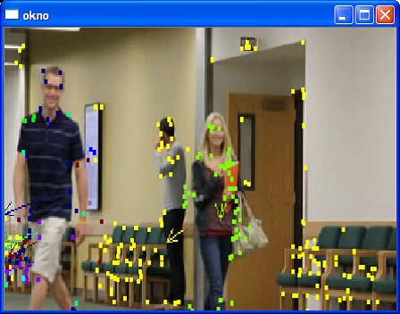
Find face/s

Facedetection in opencv is usually done by using haar cascades. You can learn more about it in opencv’s Cascade Classifier post
Code is explained there so I will skip this part.

Adjust the image for face recognition

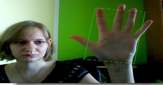
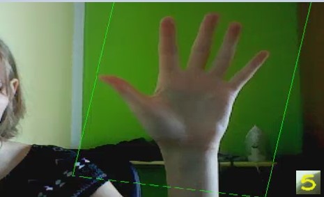
The most interesting part and the part where there is still much to do is this one. Face recognition in OpenCV works only on images with same size and greyscale. The more aligned faces are the better face recognition results are. So we need to convert the image to greyscale.


cvtColor(frame, frame_gray, CV_BGR2GRAY);

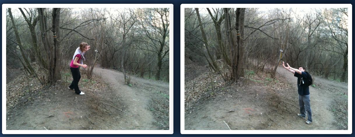
Then rotate face to vertical position so it is aligned perfectly. I do this by computing height difference between the eyes and when eyes are shut I use histogram of oriented gradients for nose to get its orientation. First thing first we need to find eyes on picture. I cropped the image to just the face part so the classifier has easier job finding eyes and doesn’t throw false positives.


int tlY = faces[i].y;
if (tlY < 0){ tlY = 0; } int drY = faces[i].y + faces[i].height; if (drY>frame.rows)
{
drY = frame.rows;
}
Point tl(faces[i].x, tlY);
Point dr(faces[i].x + faces[i].width, drY);

Rect myROI(tl, dr);
Mat croppedImage_original = frame(myROI);

I tried different crops. But the best one seems to be the one with dropped out chin and a little bit of forehead which is defaultly recognized by OpenCV’s face haar classifier. Then I use different classifier to find the eyes and I decide from x position which one is left, which one is right.


eye_cascade.detectMultiScale(croppedImageGray, eyes, 1.1, 3, CV_HAAR_DO_CANNY_PRUNING, Size(croppedImageGray.size().width*0.2, croppedImageGray.size().height*0.2));

int eyeLeftX = 0;
int eyeLeftY = 0;
int eyeRightX = 0;
int eyeRightY = 0;
for (size_t f = 0; f < eyes.size(); f++)
{
int tlY2 = eyes[f].y + faces[i].y;
if (tlY2 < 0){ tlY2 = 0; } int drY2 = eyes[f].y + eyes[f].height + faces[i].y; if (drY2>frame.rows)
{
drY2 = frame.rows;
}
Point tl2(eyes[f].x + faces[i].x, tlY2);
Point dr2(eyes[f].x + eyes[f].width + faces[i].x, drY2);

if (eyeLeftX == 0)
{

//rectangle(frame, tl2, dr2, Scalar(255, 0, 0));
eyeLeftX = eyes[f].x;
eyeLeftY = eyes[f].y;
}
else if (eyeRightX == 0)
{

////rectangle(frame, tl2, dr2, Scalar(255, 0, 0));
eyeRightX = eyes[f].x;
eyeRightY = eyes[f].y;

}

}
// if lefteye is lower than right eye swap them
if (eyeLeftX > eyeRightX){
croppedImage = cropFace(frame_gray, eyeRightX, eyeRightY, eyeLeftX, eyeLeftY, 200, 200, faces[i].x, faces[i].y, faces[i].width, faces[i].height);
}
else{
croppedImage = cropFace(frame_gray, eyeLeftX, eyeLeftY, eyeRightX, eyeRightY, 200, 200, faces[i].x, faces[i].y, faces[i].width, faces[i].height);
}

After that I rotate the face by height difference of eyes, drop it and resize it to the same size all training data is.


Mat dstImg;
Mat crop;
if (!(eyeLeftX == 0 && eyeLeftY == 0))
{

int eye_directionX = eyeRightX – eyeLeftX;
int eye_directionY = eyeRightY – eyeLeftY;
float rotation = atan2((float)eye_directionY, (float)eye_directionX) * 180 / PI;
if (rotation_def){
rotate(srcImg, rotation, dstImg);
}
else {
dstImg = srcImg;
}
}
else
{

if (noseDetection)
{
Point tl(faceX, faceY);
Point dr((faceX + faceWidth), (faceY + faceHeight));

Rect myROI(tl, dr);
Mat croppedImage_original = srcImg(myROI);

Mat noseposition_image;
resize(croppedImage_original, noseposition_image, Size(200, 200), 0, 0, INTER_CUBIC);
float rotation = gradienty(noseposition_image);
if (rotation_def){
rotate(srcImg, rotation, dstImg);
}
else {
dstImg = srcImg;
}
}
else{
dstImg = srcImg;
}

}
std::vector faces;
face_cascade.detectMultiScale(dstImg, faces, 1.1, 3, CV_HAAR_DO_CANNY_PRUNING, Size(dstImg.size().width*0.2, dstImg.size().height*0.2));

for (size_t i = 0; i < faces.size(); i++)
{

int tlY = faces[i].y;
if (tlY < 0){ tlY = 0; } int drY = faces[i].y + faces[i].height; if (drY>dstImg.rows)
{
drY = dstImg.rows;
}
Point tl(faces[i].x, tlY);
Point dr(faces[i].x + faces[i].width, drY);

Rect myROI(tl, dr);
Mat croppedImage_original = dstImg(myROI);
Mat croppedImageGray;
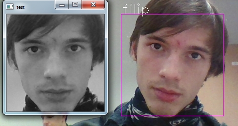
resize(croppedImage_original, crop, Size(width, height), 0, 0, INTER_CUBIC);
imshow(“test”, crop);
}

As you can see I use another face detection to find cropping area. It is probably not the best option and it is not configured for more than one face, but after few enhancements it is suffitient. The next part is rotation by nose. This is purely experimental and doesn’t give very good results. I had to use average of 4 frames to determine the rotation and it is quite slow.


int plotHistogram(Mat image)
{
Mat dst;

/// Establish the number of bins
int histSize = 256;

/// Set the ranges
float range[] = { 0, 256 };
const float* histRange = { range };

bool uniform = true; bool accumulate = false;

Mat b_hist, g_hist, r_hist;
/// Compute the histograms:
calcHist(&image, 1, 0, Mat(), b_hist, 1, &histSize, &histRange, uniform, accumulate);

int hist_w = 750; int hist_h = 500;
int bin_w = cvRound((double)hist_w / histSize);

Mat histImage(hist_h, hist_w, CV_8UC3, Scalar(0, 0, 0));

/// Normalize the result to [ 0, histImage.rows ]
normalize(b_hist, b_hist, 0, histImage.rows, NORM_MINMAX, -1, Mat());
int sum = 0;
int max = 0;
int now;
int current = 0;
for (int i = 1; i < histSize; i++)
{

now = cvRound(b_hist.at(i));
// ak su uhly v rozsahu 350-360 alebo 0-10 dame ich do suctu
if ((i < 5))
{
max += now;
current = i;
}

}

return max;

}
float gradienty(Mat frame)
{

Mat src, src_gray;
int scale = 1;
int delta = 0;
src_gray = frame;
Mat grad_x, grad_y;
Mat abs_grad_x, abs_grad_y;
Mat magnitudes, angles;
Mat bin;
Mat rotated;
int max = 0;
int uhol = 0;
for (int i = -50; i < 50; i++) { rotate(src_gray, ((double)i / PI), rotated); Sobel(rotated, grad_x, CV_32F, 1, 0, 9, scale, delta, BORDER_DEFAULT); Sobel(rotated, grad_y, CV_32F, 0, 1, 9, scale, delta, BORDER_DEFAULT); cartToPolar(grad_x, grad_y, magnitudes, angles); angles.convertTo(bin, CV_8U, 90 / PI); Point tl((bin.cols / 2) – 10, (bin.rows / 2) – 20); Point dr((bin.cols / 2) + 10, (bin.rows / 2)); Rect myROI(tl, dr); Mat working_pasik = bin(myROI); int current = 0; current = plotHistogram(working_pasik); if (current > max)
{
max = current;
uhol = i;
}
}
noseQueue.push_back(uhol);
int suma = 0;
for (std::list::iterator it = noseQueue.begin(); it != noseQueue.end(); it++)
{

suma = suma + *it;
}
int priemer;
priemer = (int)((double)suma / (double)noseQueue.size());
if (noseQueue.size() > 3)
{
noseQueue.pop_front();
}

return priemer;

}
Main idea behind this is to compute vertical and horizontal sobel for nose part and find the angle between them. Then I determine which angle is dominant with help of histogram and I use its peak value in finding the best rotation of face. This part can be improved by normalizing the histogram on start and then using just values from one face rotation angle to determine the angle between vertical position and current angle.

Rotation is done simply by this function


void rotate(cv::Mat& src, double angle, cv::Mat& dst)
{
int len = max(src.cols, src.rows);
cv::Point2f pt(len / 2., len / 2.);
cv::Mat r = cv::getRotationMatrix2D(pt, angle, 1.0);

cv::warpAffine(src, dst, r, cv::Size(len, len));
}

And in the code earlier I showed you how to crop the face and then resize it to default size.

Use trained model for face recognition

We now have model of faces trained and enhanced image of face we want to recognize. Tricky part here is determining when the face is new (not in training set) and when it is recognized properly. So I created some sort of treshold for distance and found out that it lies between 11000 and 12000.

int predictedLabel = -1;
double predicted_confidence = 0.0;
model->set("threshold", treshold);
model->predict(croppedImage, predictedLabel, predicted_confidence);

Display result

After we found out whether the person is new or not we show results:

if (predictedLabel > -1)
{

text = labels[predictedLabel];
putText(frame, text, tl, fontFace, fontScale, Scalar::all(255), thickness, 8);
}

Posted on

Saliency map

Patrik Polatsek

Introduction

Saliency model predicts what attracts the attention. The results of such models are saliency maps. A saliency map is a topographic representation of saliency which refers to visually dominant locations.

The aim of the project is to implement Itti’s saliency model. It is a hierarchical biologically inspired bottom-up model based on three features: intensity, color and orientation. The resulting saliency model is created by hierarchical decomposition of the features and their combination to the single map. Attended locations are searched using Winner-take-all neuron network.

The process

First, the features are extracted from an input image.

Intensity is obtained by converting the image to grayscale.

cvtColor( input, intensity, CV_BGR2GRAY );

For color extraction the image is converted to red-green-blue-yellow color space.

R = bgr[2] - ( bgr[1] + bgr[0] ) / 2;
G = bgr[1] - ( bgr[2] + bgr[0] ) / 2;
B = bgr[0] - ( bgr[2] + bgr[1] ) / 2;
Y = ( bgr[2] + bgr[1] ) / 2 - abs( bgr[2] - bgr[1] ) / 2 - bgr[0];

Information about local orientation is extracted using Gabor filter in four angles.

Mat kernel = getGaborKernel( Size(11, 11), 2.5, degreeToRadian(theta), 2.5, 0.5 );
filter2D( input, im, -1, kernel );

The next phase consists of creation of Gaussian pyramids.

buildPyramid( channel, pyramid, levels);

Center-surround organization of receptive field of ganglion neurons is implemented as difference-of-Gaussian between finer and coarser scales of a pyramid called a feature map.

for( int i : centerScale )
for (int i : centerScale)
{
	pyr_c = pyramid[i];
	for (int j : surroundScale)
	{
		Mat diff;
		resize(pyramid[i + j], pyr_s, pyr_c.size());
		absdiff(pyr_c, pyr_s, diff);
		differencies.push_back(diff);
	}
}

The model creates three conspicuous maps for intensity, color and orientation combining created feature maps.

The final saliency map is a mean of the conspicuous maps.

Mat saliencyMap = maps[0] / maps.size() + maps[1] / maps.size() + maps[2] / maps.size();
Saliency
Basic structure of saliency model
Posted on

LZW Coding

This is an interactive demo for LZW coding in the form of simple .NET application.

LZW Coding (Lempel–Ziv–Welch) is universal lossless data compression coding based on adaptive content-based creation of dictionary on both encoding and decoding sides.

The focus of this demo is on suitable and easy to understand visualization. The codes of dictionary entries which in reality are numbers are visualized by different colors. Single letter dictionary entries that are there from the beginning are not very interesting so all of these are represented by different shades of one color (red). Entries with more than one letter are the ones which are interesting because here is where the compression happens so these are represented by different colors to be easily distinguishable during both encoding and decoding.

Download LZW coding interactive demo

Posted on

Photo merging

Michal Lohnicky

This example shows how to merge two photos using OpenCV. SURF features are used to find a homography to align the images and histogram matching with Bhattacharyya distance is used for merging them seamlessly.

Functions used: cv.CalcHist, cv.FindHomography, cv.CompareHist(…, CV_COMP_BHATTACHARYYA), cv.ExtractSURF

Inputs

The input – two separate images

The process

  1. Preprocessing
  2. Image registration
  3. Finding the correspondences between detected points
  4. Calculating the homography
  5. Histogram matching
  6. Creating the blurred stitching mask

The matching process is demonstrated on the following images:

Detecting the SURF keypoints in both images.
Finding the correspondences between found keypoints.
The histogram calculated using Bhattacharyya distance.
The masks used to fuse both images.

Results


Python source code is provided

Posted on

Object segmentation

This example shows how to segment objects using OpenCV and Kinect for XBOX 360. The depth map retrieved from Kinect sensor is aligned with color image and used to create segmentation mask.

Functions used: convertTo, floodFill, inRange, copyTo

Inputs

The color image
The depth map

The process

  1. Retrieve color image and depth map
  2. Compute coordinates of depth map pixels so they fit to color image
  3. Align depth map with color image
    cv::Mat depth32F;
    depth16U.convertTo(depth32F, CV_32FC1);
    cv::inRange(depth32F, cv::Scalar(1.0f), cv::Scalar(1200.0f), mask);
    
  4. Find seed point in aligned depth map
  5. Perform flood fill operation from seed point
    cv::Mat mask(cv::Size(colorImageWidth + 2, colorImageHeight + 2), CV_8UC1, cv::Scalar(0));
    floodFill(depth32F, mask, seed, cv::Scalar(0.0f), NULL, cv::Scalar(20.0f), cv::Scalar(20.0f), cv::FLOODFILL_MASK_ONLY);
  6. Make a copy of color image using mask
    cv::Mat color(cv::Size(colorImageWidth, colorImageHeight), CV_8UC4, (void *) colorImageFrame->pFrameTexture, colorImageWidth * 4);
    color.copyTo(colorSegment, mask(cv::Rect(1, 1, colorImageWidth, colorImageHeight)));
    

Sample

The depth map aligned with color image
Finding the seed point
The mask – result of the flood fill operation

Result

The result of segmentation process
Posted on

TranSign, Android Sign Translator

This project shows text extraction from the input image. It is used for road sign texts translations. First, the image is preprocessed using OpenCv functions and than the text from road sign is detected and extracted.

Input

The process

  1. Image preprocessing
    Imgproc.cvtColor(img, img, Imgproc.COLOR_BGR2GRAY);
    Imgproc.GaussianBlur(img, img, new Size(5,5), 0);
    Imgproc.Sobel(img, img, CvType.CV_8U, 1, 0, 3, 1, 0);
    Imgproc.threshold(img, img, 0, 255, Imgproc.THRESH_OTSU+THRESH_BINARY);
    
  2. Contour detection
    List<MatOfPoint> contours;
    Imgproc.findContours(img, contours, new Mat(), Imgproc.RETR_EXTERNAL, Imgproc.CHAIN_APPROX_NONE);
    
  3. Deleting contours on edges, small contours, wrong ratio contours and wrong histogram contours
  4. Preprocessing before extraction
  5. Extraction
    TessBaseAPI baseApi = new TessBaseAPI();
    baseApi.init(TESSBASE_PATH, DEFAULT_LANGUAGE);
    baseApi.setImage(bm);
    String resultParcial;
    
  6. Translation

Sample

Preprocessing – converting to greyscale, Gaussian blurring, Sobel, binary threshold + Otsu’s, morphological closing
Contour detection and deleting wrong contours
Preprocessing before extraction
Extraction
Translation
Posted on

Extracting the position of game board & recognition of game board pieces

This project focuses on the usage of computer vision within the field of board games. We propose a new approach for extracting the position of game board, which consists of the detection of empty fields based on the contour analysis and elipse fitting, locating the key points by using probabilistic Hough lines and of finding the homography by using these key points.

Functions used: Canny, findContours, fitEllipse, HoughLinesP, findHomography, warpPerspective, chamerMatching

Input

The process

  1. Canny edge detector
    Mat canny;
    Canny(img, canny, 100, 170, 3);
    
  2. Contour analysis – extraction contours and filtering out those that don’t match our criteria
    vector<vector<Point>> contours;
    vector<Vec4i> hierarchy;
    findContours(canny, contours, hierarchy, CV_RETR_TREE, CV_CHAIN_APPROX_NONE);
    
  3. Ellipse fitting – further analysis of contours, final extraction of empty fields
    RotatedRect e = fitEllipse(contours[i]);
    
  4. Extraction of the game board model – 4 key points are needed for locating this model
  5. Locating the key points in the input image – using Hough lines & analysing their intersections
    Mat grayCpy;
    vector<Vec4i>& lines;
    HoughLinesP(grayCpy, lines, 1, CV_PI/180, 26, 200, 300);
    
  6. Finding the homography and final projection of the game board model into the input image
    findHomography(Mat(modelKeyPoints), Mat(keyPoints));
    warpPerspective(modelImg, newImg, h, Size(imgWithEmptyFieldsDots.cols, imgWithEmptyFieldsDots.rows), CV_INTER_LINEAR + CV_WARP_FILL_OUTLIERS);
    chamerMatching(canny, piece, results, costs, 1.0, 30, 1.0, 3, 3, 5, 0.9, 1.1);
    

Sample

Canny detector
Finding contours
Ellipse fitting I
Ellipse fitting II
Finding four key points
Probabilistic hough lines
Finding homography

Result

Projection of the game board model into the input image
Mat findImageContours(const Mat& img, vector<vector<Point> >& contours, vector<Vec4i>& hierarchy)
{
    // detect edges using canny:
    Mat canny;
    Canny(img, canny, 100, 170, 3);

    findContours(canny, contours, hierarchy, CV_RETR_TREE, CV_CHAIN_APPROX_NONE);

    // draw contours:   
    Mat imgWithContours = Mat::zeros(canny.size(), CV_8UC3);
    for (unsigned int i = 0; i < contours.size(); i++)
    {
        // process "holes" only:
        if (hierarchy[i][3] == -1) continue;
        // apply ratio + size + contourArea filters:
        if (!checkContour3(contours[i])) continue;

        // fit and draw ellipse:
        RotatedRect e = fitEllipse(contours[i]);
        if (e.size.height < 50)
        {
            line(imgWithContours, e.center, e.center, Scalar(255, 255, 255),3);
        }
    }
    return imgWithContours;
}
Posted on

Detection of map contour lines

This project shows a possible way of finding contour lines on maps. These properties of the contour lines are considered here:

  • contour lines are closed or they end at the edges of the map,
  • in some sections more neighbor contour lines are nearly parallel,
  • they are mainly slightly curved only (the lines do not have large angles like roads or buildings).

The algorithm uses the OpenCV library.

Functions used: cv::medianBlur, cv::Sobel, cv::magnitude

The process

  1. Image preprocessing – using median blur
    cv::Mat bl;
    cv::medianBlur(input, bl, params_.medianBlurKSize);
    
  2. Detecting lines and their directions – using Sobel filter (magnitudes are obtained using the magnitude function and directions are computed using atan2 from horizontal and vertical gradients)
    cv::Mat_<double> grad_x;
    cv::Sobel(beforeSobel, grad_x, CV_64F, 1, 0, params_.sobelKSize);
    cv::Sobel(beforeSobel, grad_y, CV_64F, 0, 1, params_.sobelKSize);
    
  3. Finding some contour line seeds – points at lines with approximately equal directions.
    cv::Mat_<double> magnitude;
    cv::magnitude(grad_x, grad_y, magnitude);
    
  4. Tracing lines beginning at the seeds – we are going from each seed to both directions to find the line while checking if the curves do not exceed a threshold (the more curved lines are probably not the contour lines).
  5. Filtering of the traced lines – only the lines having both ends at the image boundaries or the closed lines are considered as the map contour lines.
Input image.
Finding some contour line seeds.
Result – contour lines detected.

The result image shows a map with some contour lines detected. The seeds and line points are marked as follows:

  • yellow – seed points
  • red – closed line points
  • green – points of the first part of a line ending at the image edge
  • blue – points of the second part of a line ending at the image edge

Problems and possible improvements

These algorithm properties cause problems and need to be considered in the algorithm improvements:

  • line intersections are not being detected – one line from each pair of the intersecting lines should always be removed,
  • the algorithm uses a global magnitude threshold (the threshold determines if a point belongs to a line), but the line intensities change in most images,
  • the algorithm has too many parameters which were not generalized to match more possible images,
  • some contour lines are not continuous (they are splitted by labels) and thus not being detected by the algorithm.

Posted on

Object recognition (RANSAC verification)

This project shows object recognition using local features-based methods. We use four methods for keypoints detection and description: SIFT/SIFT, SURF/SURF, FAST/FREAK and ORB/ORB. Keypoints are used to compute homography. Object is located in scene with RANSAC algorithm. RGB and hue-saturation histograms are used for RANSAC verification.

Functions used: FeatureDetector::detect, DescriptorExtractor::compute, knnMatch, findHomography, warp, calcHist, compareHist

Input

The process

  1. Keypoints detection
    FeatureDetector * detector;
    detector = new SiftFeatureDetector();
    detector->detect( image, key_points_image );
    
    DescriptorExtractor * extractor;
    extractor = new SiftDescriptorExtractor();
    extractor->compute( image, key_points_image, des_image );
    
  2. Keypoints description
  3. Keypoints matching
    DescriptorMatcher * matcher;
    matcher = new BruteForceMatcher<L2<float>>();
    matcher->knnMatch(des_object, des_image, matches, 2);
    
  4. Calculating homography
    findHomography( obj, scene, CV_RANSAC );
    
  5. Histograms matching
    calcHist( &hsv_img_object, 1, channels, Mat(), hist_img_object, 2, histSize, ranges, true, false );
    compareHist( b_hist_object, b_hist_quad, CV_COMP_BHATTACHARYYA );
    
  6. Outline recognized object

Sample

Detecting keypoints
Finding matches
Object recognition and RANSAC verification (green outline)
Object recognition and RANSAC failure (red outline)
drawMatches( gray_object, key_points_object, image,
             key_points_image, good_matches, img_matches,
             Scalar::all(-1), Scalar::all(-1), vector<char>(),
             DrawMatchesFlags::NOT_DRAW_SINGLE_POINTS );

	if (good_matches.size() >= 4)
	{
	for( int i = 0; i < good_matches.size(); i++ )
	{
	//
	obj.push_back( key_points_object[ good_matches[i].queryIdx ].pt );
	scene.push_back( key_points_image[ good_matches[i].trainIdx ].pt );
	}

	H = findHomography( obj, scene, CV_RANSAC );

	perspectiveTransform( obj_corners, scene_corners, H);
	//*******************************************************

	Mat quad = Mat::zeros(rgb_object.rows, rgb_object.cols,
                   CV_8UC3);

	//warping object back to tamplate rotation
	warpPerspective(frame, quad, H.inv(), quad.size());

	...
Posted on

Opened and closed hand gesture detection

We detect the gesture of the opened and closed hand with sensor Kinect. State of the hand was divided into 2 parts, when it is opened (palm) or closed (fist). We assume that hand is rotated in a parallel way with the sensor and is captured her profile.

Functions used:

The process

  1. Get point in the middle of the hand and limit around her window
    Point pointHand(handFrameSize.width, handFrameSize.height);
    Rect rectHand = Rect(pos - pointHand, pos + pointHand);
    Mat depthExtractTemp = depthImageGray(rectHand); //extract hand image from depth image
    Mat depthExtract(handFrameSize.height * 2, handFrameSize.width * 2, CV_8UC1);
    

    Limiting red window with hand
  2. Find the minimum depth value in the window
    int tempDepthValue = getMinValue16(depthExtractTemp);
    
  3. Convert window from 16bit to 8bit  and use as mean value of the minimum depth
    ImageExtractDepth(&amp;depthExtractTemp, &amp;depthExtract, depthValue );
    

    Conversion 16bit to 8bit image
  4. Cut half hand in the window
    1. for the right hand from the center to the right
    2. for the left hand from the center to the left
    3. Cropping half the hand in the window
  5. Use thresholding, create mask and cut distant hand (finger)
    Mat depthThresh;
    threshold( depthThresh, depthThresh, 180, 255, CV_THRESH_BINARY_INV);
    

    Cropping half the hand in the window
  6. Determine the size of the rectangle surrounding this part of the hand
    Mat depthExtract2;
    morphologyEx(depthExtract2, depthExtract2, MORPH_CLOSE, structElement3);
    vector<vector<Point>> contours;
    vector<Vec4i> hierarchy;
    findContours(depthExtract2, contours, hierarchy, CV_RETR_EXTERNAL, CV_CHAIN_APPROX_SIMPLE, cvPoint(0,0));
    fitEllipse(Mat(contours[i]));
    
  7. If aspect ratio of width and height of the rectangle is greater than 1, then hand is opened, else hand is closed

    Right hand shape and left detection rectangle

Limitation

  • Maximal distance detection is 2 meters
  • Maximal slope hand is up or down by 25 degrees
  • Profile of hand must be turned parallel with the sensor

Result

Detection of both hand (right and left) takes 4ms.

Opened and closed hand
Augmented Reality with hand detection
Posted on

Tracking people in video with calculating the average speed of the monitored points

This example shows a new method for tracking significant points in video, representing people or moving objects. This method uses several OpenCV functions.

The process

  1. The opening video file
    VideoCapture MojeVideo („cesta k súboru");
    
  2. Retrieve the next frame (picture)
    Mat FarebnaSnimka;
    MojeVideo >> FarebnaSnimka;
    
  3. Converting color images to grayscale image
    Mat Snimka1;
    cvtColor(FarebnaSnimka, Snimka1, CV_RGB2GRAY);
    
  4. Getting significant (well observable) points
    vector<cv::Point2f> VyznacneBody;
    goodFeaturesToTrack(Snimka1, VyznacneBody, 300, 0.06, 0);
    
  5. Getting the next frame and its conversion
  6. Finding significant points from the previous frame to the next
    vector<cv::Point2f> PosunuteBody;
    vector<uchar> PlatneBody;
    calcOpticalFlowPyrLK(Snimka1, Snimka2, VyznacneBody, PosunuteBody, PlatneBody, err);
    
  7. Calculation of the velocity vector for each significant point
  8. Clustering of significant points according to their average velocity vectors
  9. Visualization
    1. Assign a color to cluster
    2. Plotting points on a slide
    3. Plotting arrows at the center points of clusters – average of the average velocity vectors
  10. Dumping the clusters and other places for the classification of points into them (to preserve the color of the cluster) + eventual creation of new clusters
  11. Landmarks declining over time – the time when they need to re-designate

Result

  • This method is faster than OpenCV method for detecting people.
  • It also works when only part of person is visible, position is unusual or person is rotated.
  • Person is divided to parts.
  • It does not distinguish between persons or other moving objects.