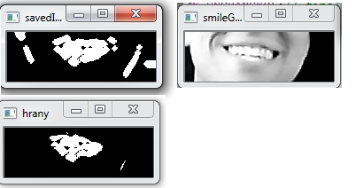
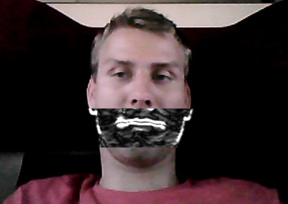
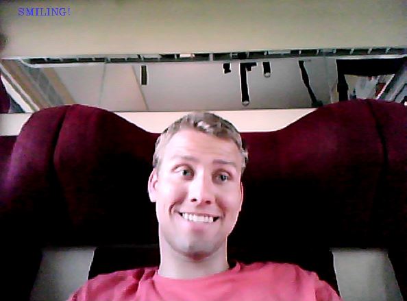
Smile detection is a popular feature of today’s photo cameras. It is not implemented in all cameras, as a popular face detection, because it is more complicated to implement. This project shows a basic algorihtm in the topic. It may be used but few improvements are necessary. Sobel filter and thresholding are used. There is a mask which is compared to every filtered image from a webcam. If the images are more than 60% equal, smile is detected. Used Functions detectMultiScale, Sobel, medianBlur, threshold, dilate, bitwise_and
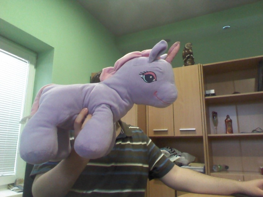
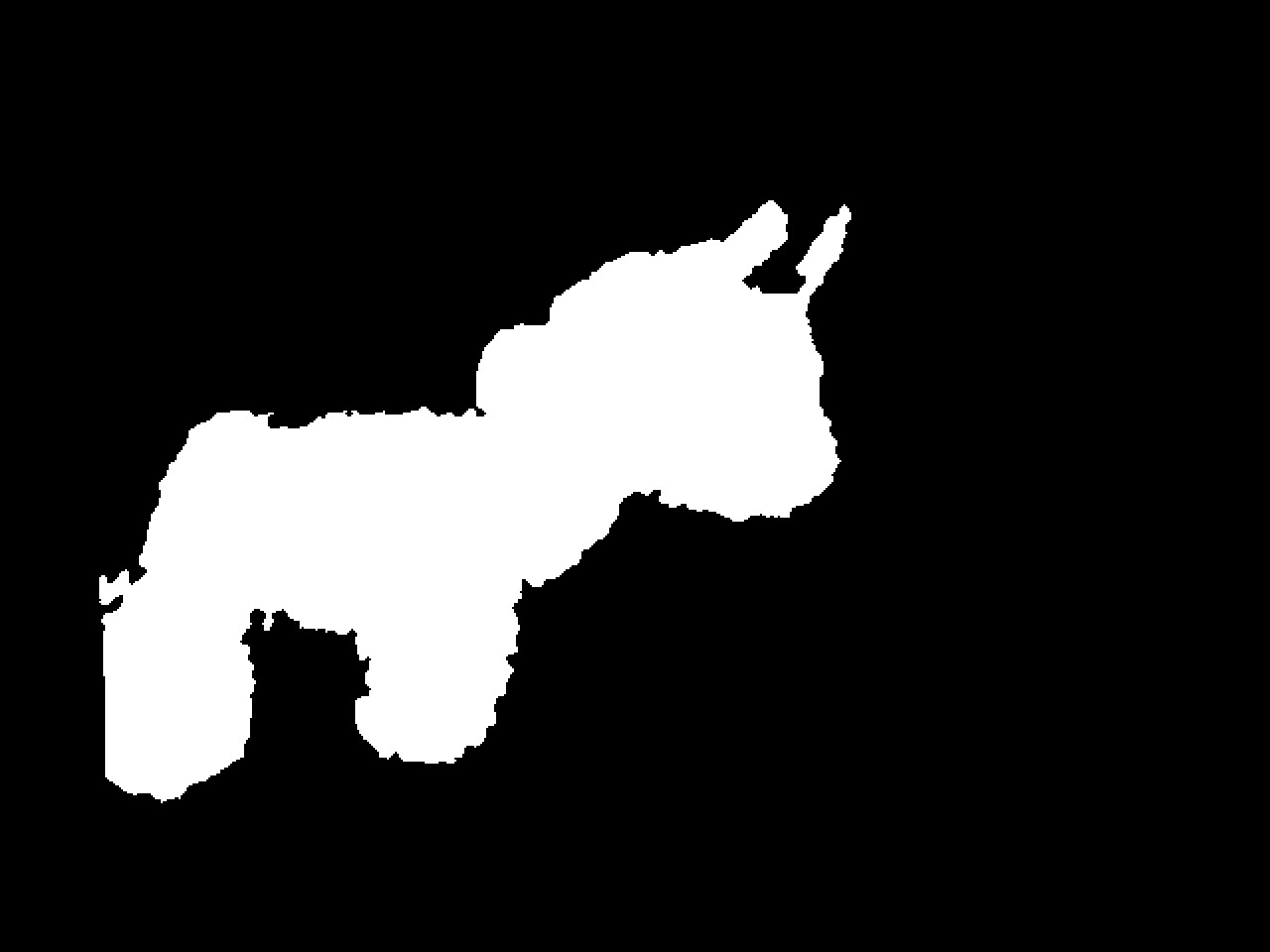
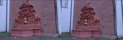
In this example we focus on enhancing the current SIFT descriptor vector with additional two dimensions using depth map information obtained from kinect device. Depth map is used for object segmentation (see: http://vgg.fiit.stuba.sk/2013-07/object-segmentation/) as well to compute standard deviation and the difference of minimal and maximal distance from surface around each of detected keypoints. Those two metrics are used to enhance SIFT descriptor.
To be able to enhance SIFT descriptor and still provide good matching results, we need to evaluate the precision of selected metrics. We have chosen to visualize the normal vectors computed from the surface around keypoints.
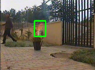
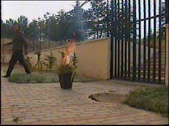
The main aim of this example is to automatically detect fire in video, using computer vision methods, implemented in real-time with the aid of the OpenCV library. Proposed solution must be applicable in existing security systems, meaning with the use of regular industrial or personal video cameras. Necessary solution precondition is that camera is static. Given the computer vision and image processing point of view, stated problem corresponds to detection of dynamically changing object, based on his color and moving features.
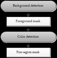
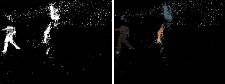
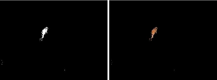
While static cameras are utilized, background detection method provides effective segmentation of dynamic objects in video sequence. Candidate fire-like regions of segmented foreground objects are determined according to the rule-based color detection.
Input
Process outline
Process steps
Retrieve current video frame
capture.retrieve(frame);
Update background model and save foreground mask to
BackgroundSubtractorMOG2 pMOG2;
Mat fgMaskMOG2,
pMOG2(frame, fgMaskMOG2);
Convert current 8-bit frame in RGB color space to 32-bit floating point YCbCr color space.
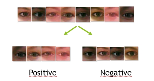
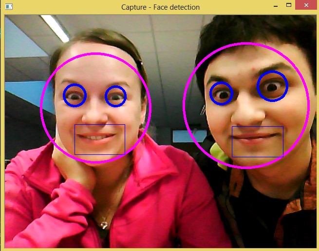
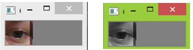
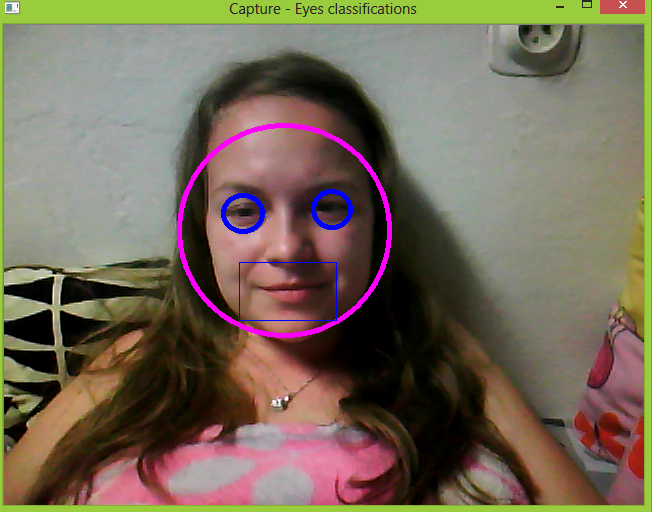
The project shows detection and recognition of face and eyes from input image (webcam). I use for detection and classification haarcascade files from OpenCV. If eyes are recognized, I classify them as opened or narrowed. The algorithm uses the OpenCV andSVMLight library.
As first I make positive and negative dataset. Positive dataset are photos of narrowed eyes and negative dataset are photos of opened eyes.
Then I make HOGDescriptor and I use it to compute feature vector for every picture. These pictures are used to train SVM vector and their feature vectors are saved to one file: features.dat
I detect every face and every eye from picture. For every found picture of eye I cut it and I use HOGDescriptor to detect narrowed shape of eye.
Face, Eye and Mouth detectionCutting eyes and conversion to grayscale format
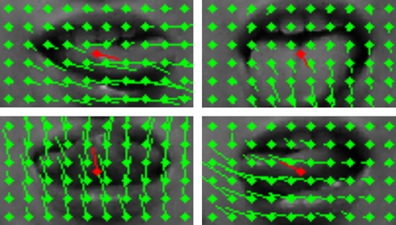
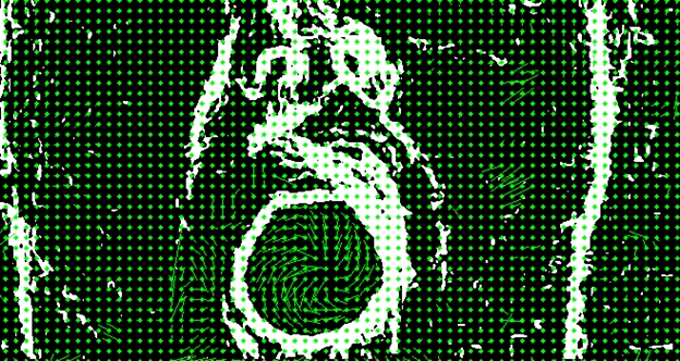
This project is focused on tracking tongue using just the information from plain web camera. Â Majority of approaches tried in this project failed including edge detection, morphological reconstruction and point tracking because of various reasons like homogenous and position-variable character of tongue.
The approach that yields usable results is Farneback method of optical flow. By using this method we are able to detect the direction of movement in image and tongue specifically when we use it on image of sole mouth. However mouth area found by haar cascade classifier is very shaky so the key part is to stabilize it.
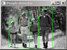
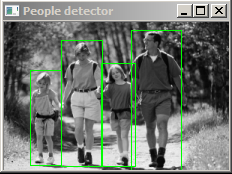
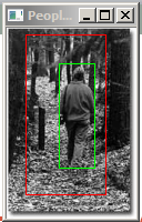
The goal of this project is detection of people on images. Persons on images are:
standing
person can be rotated from the front, back and from the side
different sizes of persons
can be in move
several persons on single image
For our project the main challenge was the highest possible precision of detection, detection of all persons on image in all possible situations. Persons can also be interleaved.
In our project we have experimented with two different approaches. Both are based on SVM classifier. This classifier takes images as input and detects persons on image. HOG descriptor is used by classifier to extract features from images in classification process. Sliding window is used to detect persons of different sizes. We have experimented with two different classifiers on two different datasets (D1 and D2).
Trained classifier from OpenCV
Precision:
D1: 51.5038%, 3 false positives
D2: 56.3511%, 49 false positives
Our trained classifier
Precision
D1: 66.9556%, 87 false positives
D2: 40.4521%, 61 false positives
Result of people detection:
We see possible improvments in extracting other features from images, or in using bigger datasets.
void App::trainSVM()
{
	CvSVMParams params;
	/*params.svm_type = CvSVM::C_SVC;
	params.kernel_type = CvSVM::LINEAR;
	params.term_crit = cvTermCriteria(CV_TERMCRIT_ITER, 100, 1e-6);*/
	params.svm_type = SVM::C_SVC;
	params.C = 0.1;
	params.kernel_type = SVM::LINEAR;
	params.term_crit = TermCriteria(CV_TERMCRIT_ITER, (int)1e7, 1e-6);
	int rows = features.size();
	int cols = number_of_features();
	Mat featuresMat(rows, cols, CV_32FC1);
	Mat labelsMat(rows, 1, CV_32FC1);
	for (unsigned i = 0; i<rows; i++)
	{
		for (unsigned j = 0; j<cols; j++)
		{
			featuresMat.at<float>(i, j) = features.at(i).at(j);
		}
	}
	for (unsigned i = 0; i<rows; i++)
	{
		labelsMat.at<float>(i, 0) = labels.at(i);
	}
	SVM.train(featuresMat, labelsMat, Mat(), Mat(), params);
	SVM.getSupportVector(trainedDetector);
	hog.setSVMDetector(trainedDetector);
}
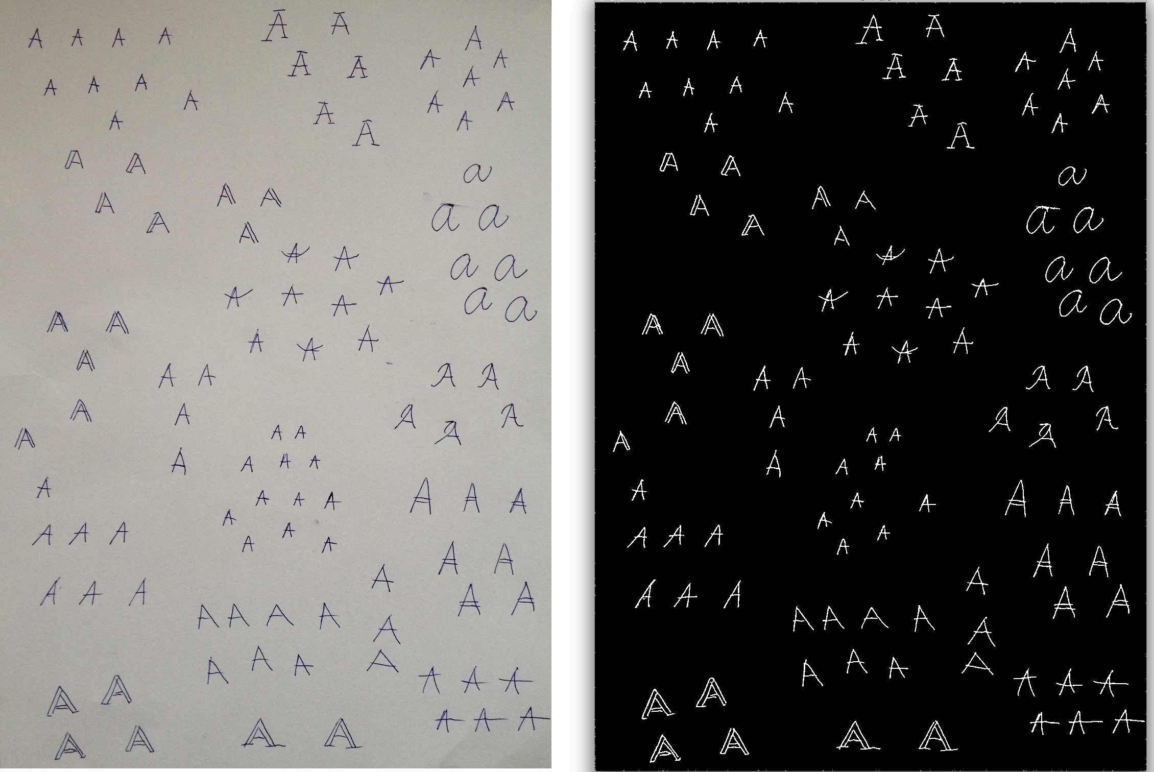
Example down below shows conversion of scanned or photographed images of typewritten text into machine-encoded/computer-readable text. Process was divided into pre-processing, learning and character recognizing. Algorithm is implemented using the OpenCV library and C++.
 The process
Pre-processing – grey-scale, median blur, adaptive threshold, closing
Learning – we need image with different written styles of same character for each character we want to recognizing. For each reference picture we use these methods: findContours, detect too small areas and remove them from picture.
vector < vector<Point> > contours;
vector<Vec4i> hierarchy;
findContours(result, contours, hierarchy, CV_RETR_CCOMP,
	CV_CHAIN_APPROX_SIMPLE);
for (int i = 0; i < contours.size(); i = hierarchy[i][0]) {
	Rect r = boundingRect(contours[i]);
	double area0 = contourArea(contours[i]);
	if (area0 < 120) {
		drawContours(thr, contours, i, 0, CV_FILLED, 8, hierarchy);
		continue;
	}
}
Next step is to resize all contours to fixed size 50×50 and save as new png image.
We get folder for each character with 50×50 images
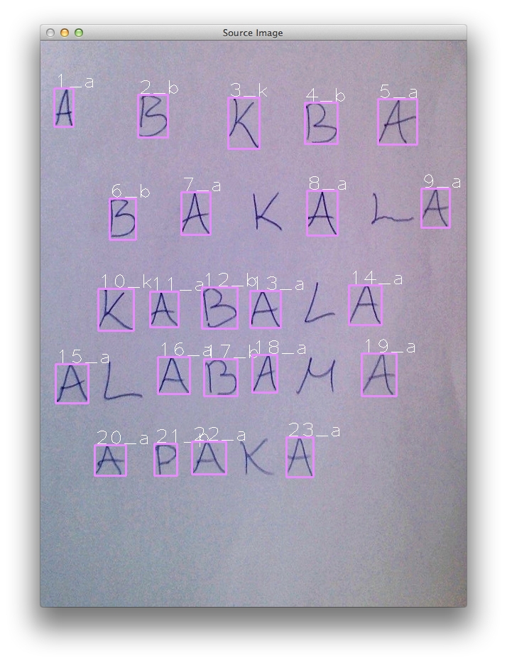
Recognizing – now we know what look like A, B, C … For recognition of each character in our picture we use steps from previous state of algorithm. We pre-process our picture find contour and get rid of small areas. Next step is to order contours that we can easily output characters in right order.
while (rectangles.size() > 0) {
	vector<Rect> pom;
	Rect min = rectangles[rectangles.size() - 1];
	for (int i = rectangles.size() - 1; i >= 0; i--) {
		if ((rectangles[i].y < (min.y + min.height / 2)) && (rectangles[i].y >(min.y - min.height / 2))) {
			pom.push_back(rectangles[i]);
			rectangles.erase(rectangles.begin() + i);
		}
	}
	results.push_back(pom);
}
Template matching is method for match two images, where template is each of our 50×50 images from learning state and next image is ordered contour.
foreach detected in image
	foreach template in learned
		if detected == template
			break
		end
	end
end
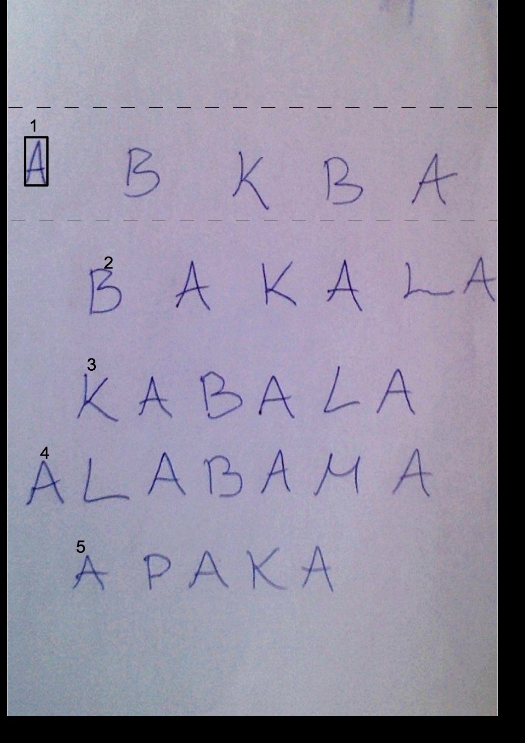
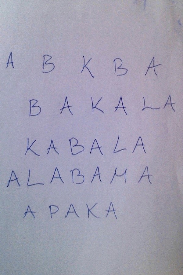
Results
Recognizing characters with template matching in ordered contours array where templates are our learned images of characters. Contours images have to be resize to 51×51 pixels because our templates are 50×50 pixels.
matchTemplate(ROI, tpl, result, CV_TM_SQDIFF_NORMED);
minMaxLoc(result, &minVal, &maxVal, &minLoc, &maxLoc, Mat());
if (maxVal >= 0.9) {	//treshold
	cout << name; // print character
	found = true;
	return true;
}
Currently we support only characters A, B, K. We can see that character K was recognized twice from 4 characters in image. That’s because out set of K written styles was too small (12 pictures). Recognition of characters A and B was 100 % successful (set has 120 written style pictures).
In this project, we aim to recognize the gestures made by the users by moving their lips; Examples: closed mouth, mouth open, mouth wide open, puckered lips. The challenges in this task are the high homogeneity in the observed area, and the rapidity of lip movements. Our first attempts in detecting said gestures are based on the detection of the lip movements through flow with the Farneback method implemented in OpenCV, or alternatively the calculation of the motion gradient from a silhouette image. It appears, that these methods might not be optimal for the solution of this problem.
Detect the position of the largest face in the image using OpenCV cascade classifier. Further steps will be applied using the lower half of the found face.
faceRects = detect(frame, faceClass);
Transform the image map to HLS color space, and obtain the luminosity map of the image
Combine the results of horizontal and vertical Sobel methods to detect edges of the face features.
Add accumulative edge detection frame images on top of each other to obtain the silhouette image. To prevent raised noise in areas without edges, apply a threshold to the Sobel map.
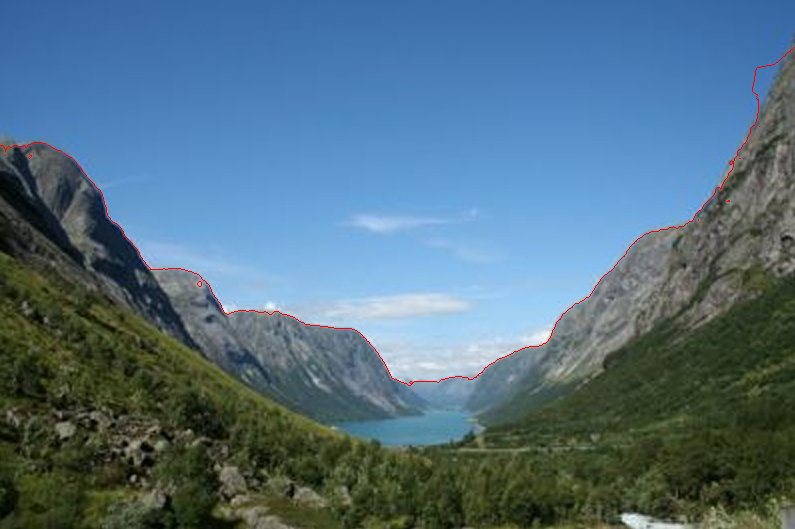
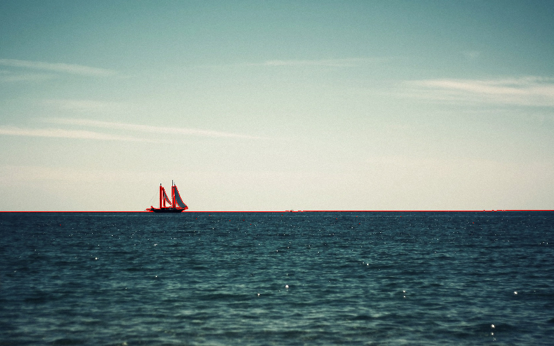
This project tries to solve the problem of sky detection using the Slic superpixel segmentation algorithm.
Analysis
The first idea was to use Slic superpixel algorithm to segment an input image and merge pairs of adjecent superpixels based on their similarity. We created a simple tool to manually evaluate the hypothesis that a sky can be separated from a photo with one threshold. In this prototype, we compute the similarity between superpixels as an Euclidean distance between their mean colors in the RGB color space. For the most of images from our dataset we found a threshold which can be used for sky segmentation process.
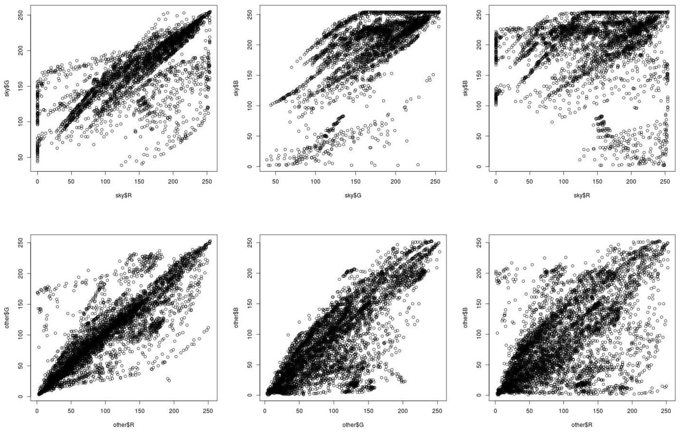
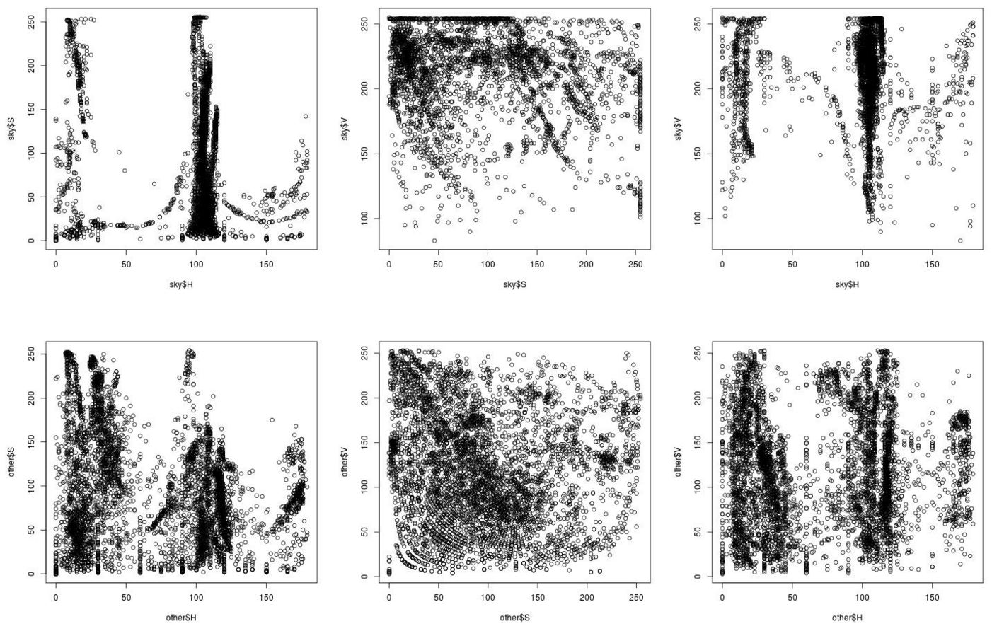
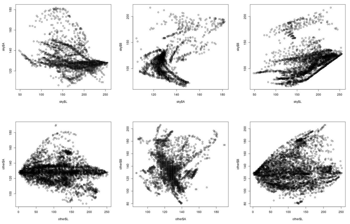
Next, we analyzed colors of images from our dataset. For each image we saved superpixel colors for sky and the rest of the image in three color spaces (RGB, HSV and Lab) and we plotted them. The resulting graphs are shown below (the first row of graphs represents sky colors, the second row represents colors of the rest of an image). As we can see, the biggest difference is in HSV an Lab color spaces. Based on this evaluation, we choosed Lab as a base working color space to compare superpixels.
RGB
HSV
Lab
Final algorithm
Generating superpixels using Slic algorithm
Replacing superpixels with their mean color values
Setting threshold:
T = [ d1 + (d2 - d1) * 0.3 ] * 1.15
where:
d1 – average distance between superpixels in the top 10% of an image
d2 – average distance between superpixels in an image without â…“ smallest distances
The values 0,3 and 1,15 was choosed for best (universal) results for our dataset.
Merging adjecent superpixels
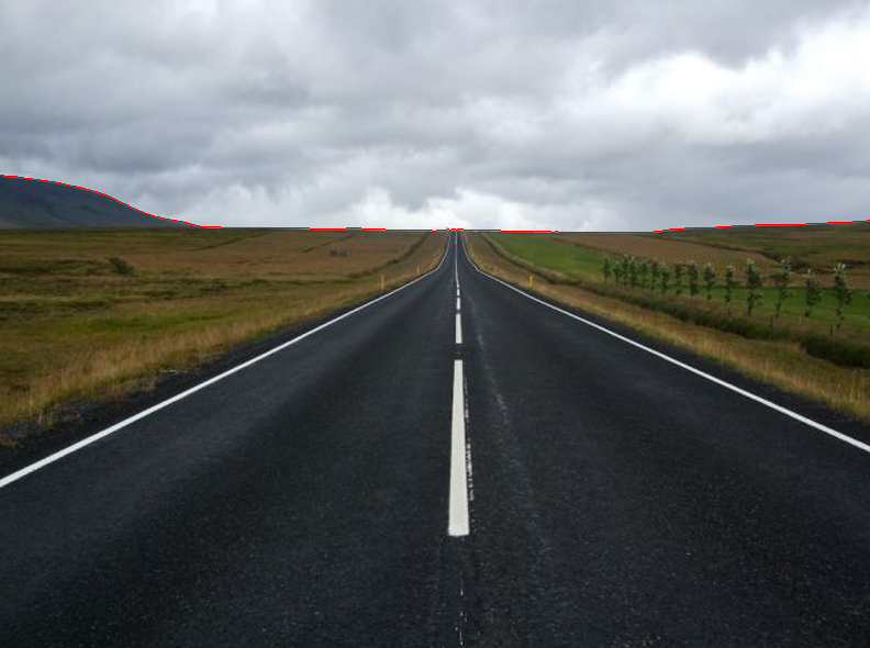
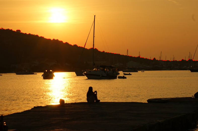
Choosing sky – superpixel with the largest number of pixels in the first row
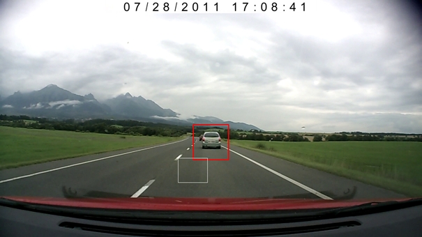
This project started with car detection using Haar Cascade Classifier. Then we focused on eliminating false positive results by using road detection. We tested the solution on a recorded video, which was obtained with a car camera recorder.
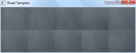
Capture road sample every n-th frame, by capturing rectangle positioned statically in the frame (white rectangle in the examples). Road sample shouldn’t contain line markings. We used canny and countNonZero to avoid line marking.
Road samples
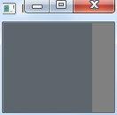
Calculate average road color from captured road samples
Average road color
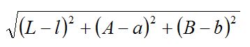
Convert image and average road sample to LAB color space.
For each pixel from the input image, calculate:
where L, A, B are values from the input image and l, a, b are values from average road sample.
Binarize the result by using threshold function.
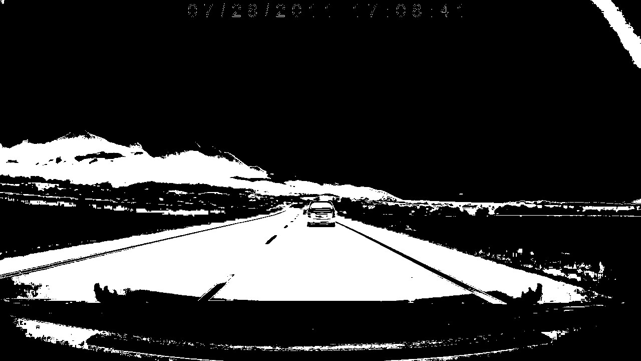
Example
Input image, car detected is in red rectangleRoad detection
Bag of visual words (BOW) representation was based on Bag of words in text processing. This method requires following for basic user:
Image dataset splitted into image groups, or
precomputed image dataset and group histogram representation stored in .xml or .yml file (see XML/YAML Persistence chapter in OpenCV documentation)
at least one image to compare via BOW
Image dataset is stored in folder (of any name) with subfolders named by group names. In the subfolders there are images for current group stored. BOW should generate and store descriptors and histograms into specified output .xml or .yml file.
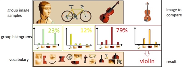
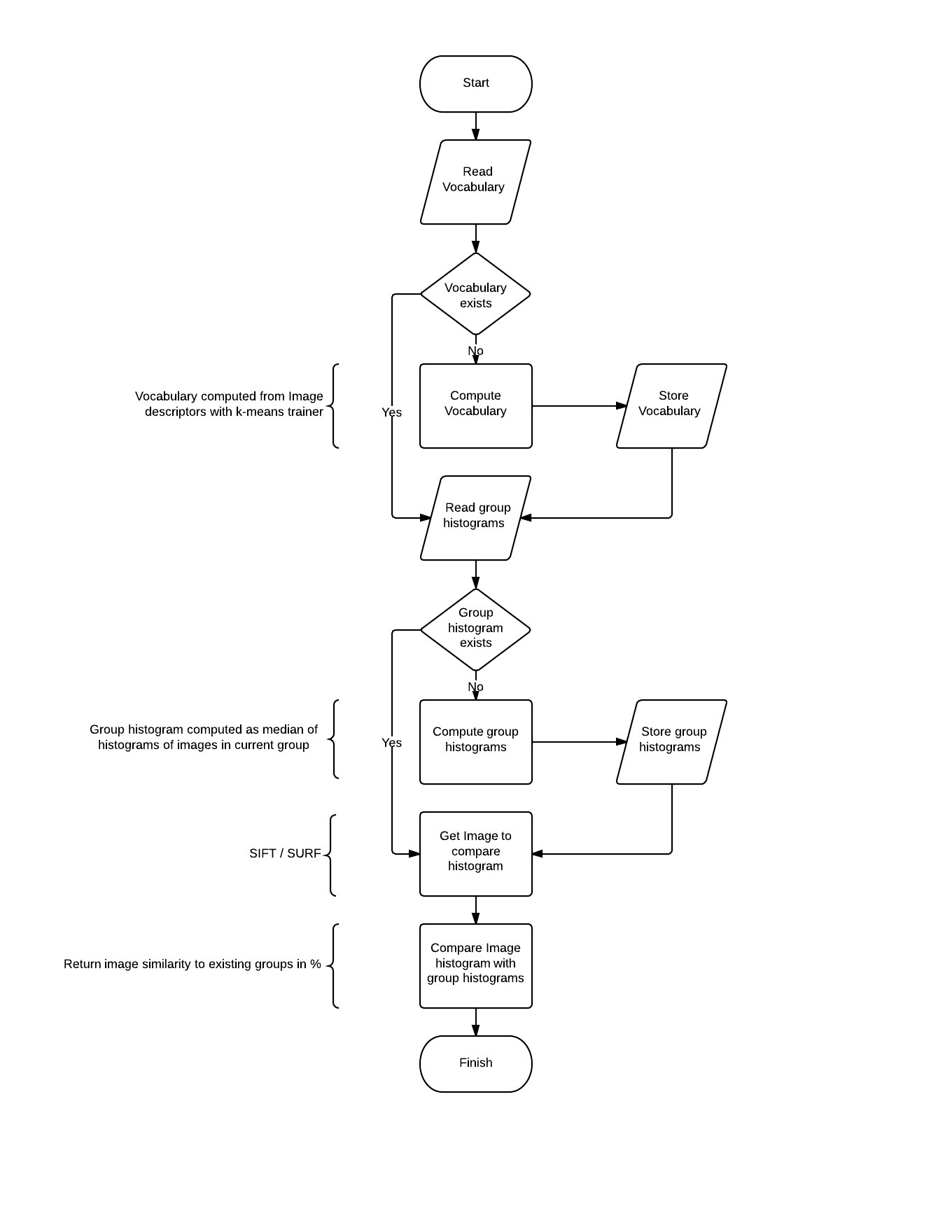
BOW works as follows (compare with Figure 1 and 2):
compute visual word vocabulary with k-means algorithm (where k is equivalent with count of visual words in vocabulary). Vocabulary is stored into output file. This should take about 30 minutes on 8 CPU cores when k=500 and image count = 150. OpenMP is used to improve performance.
compute group histograms (there are 2 methods implemented for this purpose – median and average histogram, only median is used because of better results). This part requires vocabulary computed. Group histogram is normalized histogram, this means sum of all columns within the histogram equals 1.
compute histogram for picture on input and compare it with all group histograms to realize which group image belongs to. This was implemented as histogram intersection.
As seen in Figure 2, whole vocabulary and group histogram computation may be skipped if they were already computed.
Figure 1: BOW tacticFigure 2: Flowchart for whole BOW implementation
For usage simplification I have implemented BOWProperties class as singleton, which holds basic information and settings like BOWDescriptorExtractor, BOWTrainer, reading images as grayscaled images or method for obtaining descriptors (SIFT and SURF are currently implemented and ready to use). Example of implementation is here:
BOWProperties* BOWProperties::setFeatureDetector(const string type, int featuresCount)
{
	Ptr<FeatureDetector> featureDetector;
	if (type.compare(SURF_TYPE) == 0)
	{
		if (featuresCount == UNDEFINED) featureDetector = new SurfFeatureDetector();
		else featureDetector = new SurfFeatureDetector(featuresCount);
	}
	...
}
This is how all other properties are set. The only thing that user have to do is simply set properties and run classification.
There is in most cases single DataSet object holding reference to groups and some Group objects that holds references to images in the group in my implementation. Training implementation:
DataSet part :
void DataSet::trainBOW()
{
	BOWProperties* properties = BOWProperties::Instance();
	Mat vocabulary;
	// read vocabulary from file if not exists compute it
	if (!Utils::readMatrix(properties->getMatrixStorage(), vocabulary, "vocabulary"))
	{
		for each (Group group in groups)
			group.trainBOW();
		vocabulary = properties->getBowTrainer()->cluster();
		Utils::saveMatrix(properties->getMatrixStorage(), vocabulary, "vocabulary");
	}
	BOWProperties::Instance()
		->getBOWImageDescriptorExtractor()
		->setVocabulary(vocabulary);
}
Group part (notice OpenMP usage for parallelization):
unsigned Group::trainBOW()
{
	unsigned descriptor_count = 0;
	Ptr<BOWKMeansTrainer> trainer = BOWProperties::Instance()->getBowTrainer();

	#pragma omp parallel for shared(trainer, descriptor_count)
	for (int i = 0; i < (int)images.size(); i++){
		Mat descriptors = images[i].getDescriptors();
		#pragma omp critical
		{
			trainer->add(descriptors);
			descriptor_count += descriptors.rows;
		}
	}
	return descriptor_count;
}
This part of code generates and stores vocabulary. The getDescriptors() method returns descriptors for current image via DescriptorExtractor class. Next part shows how the group histograms are computed:
Where getMedianHistogram() method generates median histogram from histograms that are representing each image in current group.
Now the vocabulary and histogram classifiers are computed and stored. Last part is comparing new image with the classifiers.
Group DataSet::getImageClass(Image image)
{
	for (int i = 0; i < groups.size(); i++)
	{
		currentFit = Utils::getHistogramIntersection(groups[i].getGroupClasifier(), image.getHistogram());
		if (currentFit > bestFit){
			bestFit = currentFit;
			bestFitPos = i;
		}
	}
	return groups[bestFitPos];
}
The returned group is group where image most possibly belongs. Nearly every piece of code is little bit simplified but shows basic thoughts. For more detailed code, see sources.
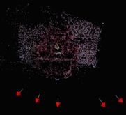
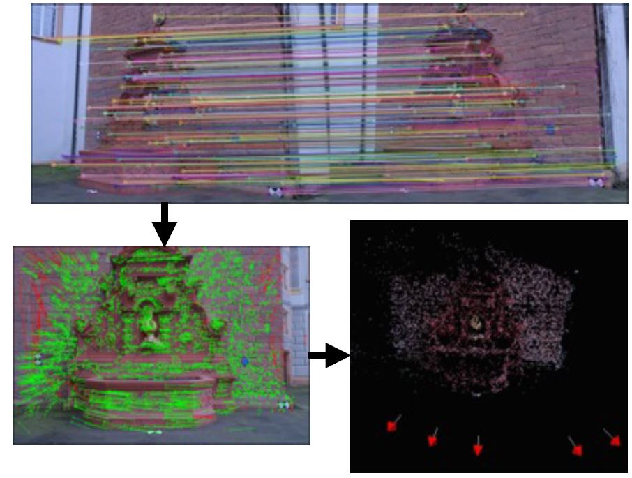
Main objective of this project was to reconstruct the 3D scene from set of images or recorded video. First step is to find relevant matches between two related images and use this matches to calculate rotation and translation of camera for each input image or frame. In final stage the depth value is extracted with triangulation algorithm.
We have successfully extracted the depth value for each relevant matching point. But we were not able to visualise the result because of the PCL and other external libraries. In future we try to use Matlab to validate our result.