Posted on

Object segmentation

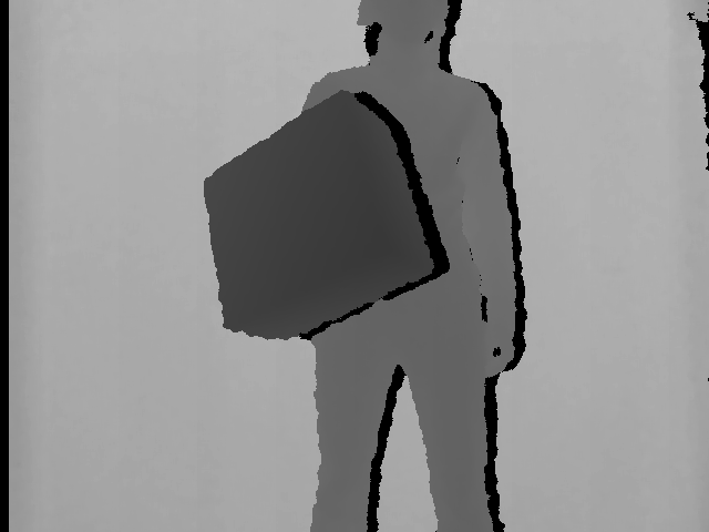
This example shows how to segment objects using OpenCV and Kinect for XBOX 360. The depth map retrieved from Kinect sensor is aligned with color image and used to create segmentation mask.

Functions used: convertTo, floodFill, inRange, copyTo

Inputs

The color image
The depth map

The process

  1. Retrieve color image and depth map
  2. Compute coordinates of depth map pixels so they fit to color image
  3. Align depth map with color image
    cv::Mat depth32F;
    depth16U.convertTo(depth32F, CV_32FC1);
    cv::inRange(depth32F, cv::Scalar(1.0f), cv::Scalar(1200.0f), mask);
    
  4. Find seed point in aligned depth map
  5. Perform flood fill operation from seed point
    cv::Mat mask(cv::Size(colorImageWidth + 2, colorImageHeight + 2), CV_8UC1, cv::Scalar(0));
    floodFill(depth32F, mask, seed, cv::Scalar(0.0f), NULL, cv::Scalar(20.0f), cv::Scalar(20.0f), cv::FLOODFILL_MASK_ONLY);
  6. Make a copy of color image using mask
    cv::Mat color(cv::Size(colorImageWidth, colorImageHeight), CV_8UC4, (void *) colorImageFrame->pFrameTexture, colorImageWidth * 4);
    color.copyTo(colorSegment, mask(cv::Rect(1, 1, colorImageWidth, colorImageHeight)));
    

Sample

The depth map aligned with color image
Finding the seed point
The mask – result of the flood fill operation

Result

The result of segmentation process
Posted on

TranSign, Android Sign Translator

This project shows text extraction from the input image. It is used for road sign texts translations. First, the image is preprocessed using OpenCv functions and than the text from road sign is detected and extracted.

Input

The process

  1. Image preprocessing
    Imgproc.cvtColor(img, img, Imgproc.COLOR_BGR2GRAY);
    Imgproc.GaussianBlur(img, img, new Size(5,5), 0);
    Imgproc.Sobel(img, img, CvType.CV_8U, 1, 0, 3, 1, 0);
    Imgproc.threshold(img, img, 0, 255, Imgproc.THRESH_OTSU+THRESH_BINARY);
    
  2. Contour detection
    List<MatOfPoint> contours;
    Imgproc.findContours(img, contours, new Mat(), Imgproc.RETR_EXTERNAL, Imgproc.CHAIN_APPROX_NONE);
    
  3. Deleting contours on edges, small contours, wrong ratio contours and wrong histogram contours
  4. Preprocessing before extraction
  5. Extraction
    TessBaseAPI baseApi = new TessBaseAPI();
    baseApi.init(TESSBASE_PATH, DEFAULT_LANGUAGE);
    baseApi.setImage(bm);
    String resultParcial;
    
  6. Translation

Sample

Preprocessing – converting to greyscale, Gaussian blurring, Sobel, binary threshold + Otsu’s, morphological closing
Contour detection and deleting wrong contours
Preprocessing before extraction
Extraction
Translation
Posted on

Extracting the position of game board & recognition of game board pieces

This project focuses on the usage of computer vision within the field of board games. We propose a new approach for extracting the position of game board, which consists of the detection of empty fields based on the contour analysis and elipse fitting, locating the key points by using probabilistic Hough lines and of finding the homography by using these key points.

Functions used: Canny, findContours, fitEllipse, HoughLinesP, findHomography, warpPerspective, chamerMatching

Input

The process

  1. Canny edge detector
    Mat canny;
    Canny(img, canny, 100, 170, 3);
    
  2. Contour analysis – extraction contours and filtering out those that don’t match our criteria
    vector<vector<Point>> contours;
    vector<Vec4i> hierarchy;
    findContours(canny, contours, hierarchy, CV_RETR_TREE, CV_CHAIN_APPROX_NONE);
    
  3. Ellipse fitting – further analysis of contours, final extraction of empty fields
    RotatedRect e = fitEllipse(contours[i]);
    
  4. Extraction of the game board model – 4 key points are needed for locating this model
  5. Locating the key points in the input image – using Hough lines & analysing their intersections
    Mat grayCpy;
    vector<Vec4i>& lines;
    HoughLinesP(grayCpy, lines, 1, CV_PI/180, 26, 200, 300);
    
  6. Finding the homography and final projection of the game board model into the input image
    findHomography(Mat(modelKeyPoints), Mat(keyPoints));
    warpPerspective(modelImg, newImg, h, Size(imgWithEmptyFieldsDots.cols, imgWithEmptyFieldsDots.rows), CV_INTER_LINEAR + CV_WARP_FILL_OUTLIERS);
    chamerMatching(canny, piece, results, costs, 1.0, 30, 1.0, 3, 3, 5, 0.9, 1.1);
    

Sample

Canny detector
Finding contours
Ellipse fitting I
Ellipse fitting II
Finding four key points
Probabilistic hough lines
Finding homography

Result

Projection of the game board model into the input image
Mat findImageContours(const Mat& img, vector<vector<Point> >& contours, vector<Vec4i>& hierarchy)
{
    // detect edges using canny:
    Mat canny;
    Canny(img, canny, 100, 170, 3);

    findContours(canny, contours, hierarchy, CV_RETR_TREE, CV_CHAIN_APPROX_NONE);

    // draw contours:   
    Mat imgWithContours = Mat::zeros(canny.size(), CV_8UC3);
    for (unsigned int i = 0; i < contours.size(); i++)
    {
        // process "holes" only:
        if (hierarchy[i][3] == -1) continue;
        // apply ratio + size + contourArea filters:
        if (!checkContour3(contours[i])) continue;

        // fit and draw ellipse:
        RotatedRect e = fitEllipse(contours[i]);
        if (e.size.height < 50)
        {
            line(imgWithContours, e.center, e.center, Scalar(255, 255, 255),3);
        }
    }
    return imgWithContours;
}
Posted on

Detection of map contour lines

This project shows a possible way of finding contour lines on maps. These properties of the contour lines are considered here:

  • contour lines are closed or they end at the edges of the map,
  • in some sections more neighbor contour lines are nearly parallel,
  • they are mainly slightly curved only (the lines do not have large angles like roads or buildings).

The algorithm uses the OpenCV library.

Functions used: cv::medianBlur, cv::Sobel, cv::magnitude

The process

  1. Image preprocessing – using median blur
    cv::Mat bl;
    cv::medianBlur(input, bl, params_.medianBlurKSize);
    
  2. Detecting lines and their directions – using Sobel filter (magnitudes are obtained using the magnitude function and directions are computed using atan2 from horizontal and vertical gradients)
    cv::Mat_<double> grad_x;
    cv::Sobel(beforeSobel, grad_x, CV_64F, 1, 0, params_.sobelKSize);
    cv::Sobel(beforeSobel, grad_y, CV_64F, 0, 1, params_.sobelKSize);
    
  3. Finding some contour line seeds – points at lines with approximately equal directions.
    cv::Mat_<double> magnitude;
    cv::magnitude(grad_x, grad_y, magnitude);
    
  4. Tracing lines beginning at the seeds – we are going from each seed to both directions to find the line while checking if the curves do not exceed a threshold (the more curved lines are probably not the contour lines).
  5. Filtering of the traced lines – only the lines having both ends at the image boundaries or the closed lines are considered as the map contour lines.
Input image.
Finding some contour line seeds.
Result – contour lines detected.

The result image shows a map with some contour lines detected. The seeds and line points are marked as follows:

  • yellow – seed points
  • red – closed line points
  • green – points of the first part of a line ending at the image edge
  • blue – points of the second part of a line ending at the image edge

Problems and possible improvements

These algorithm properties cause problems and need to be considered in the algorithm improvements:

  • line intersections are not being detected – one line from each pair of the intersecting lines should always be removed,
  • the algorithm uses a global magnitude threshold (the threshold determines if a point belongs to a line), but the line intensities change in most images,
  • the algorithm has too many parameters which were not generalized to match more possible images,
  • some contour lines are not continuous (they are splitted by labels) and thus not being detected by the algorithm.

Posted on

Object recognition (RANSAC verification)

This project shows object recognition using local features-based methods. We use four methods for keypoints detection and description: SIFT/SIFT, SURF/SURF, FAST/FREAK and ORB/ORB. Keypoints are used to compute homography. Object is located in scene with RANSAC algorithm. RGB and hue-saturation histograms are used for RANSAC verification.

Functions used: FeatureDetector::detect, DescriptorExtractor::compute, knnMatch, findHomography, warp, calcHist, compareHist

Input

The process

  1. Keypoints detection
    FeatureDetector * detector;
    detector = new SiftFeatureDetector();
    detector->detect( image, key_points_image );
    
    DescriptorExtractor * extractor;
    extractor = new SiftDescriptorExtractor();
    extractor->compute( image, key_points_image, des_image );
    
  2. Keypoints description
  3. Keypoints matching
    DescriptorMatcher * matcher;
    matcher = new BruteForceMatcher<L2<float>>();
    matcher->knnMatch(des_object, des_image, matches, 2);
    
  4. Calculating homography
    findHomography( obj, scene, CV_RANSAC );
    
  5. Histograms matching
    calcHist( &hsv_img_object, 1, channels, Mat(), hist_img_object, 2, histSize, ranges, true, false );
    compareHist( b_hist_object, b_hist_quad, CV_COMP_BHATTACHARYYA );
    
  6. Outline recognized object

Sample

Detecting keypoints
Finding matches
Object recognition and RANSAC verification (green outline)
Object recognition and RANSAC failure (red outline)
drawMatches( gray_object, key_points_object, image,
             key_points_image, good_matches, img_matches,
             Scalar::all(-1), Scalar::all(-1), vector<char>(),
             DrawMatchesFlags::NOT_DRAW_SINGLE_POINTS );

	if (good_matches.size() >= 4)
	{
	for( int i = 0; i < good_matches.size(); i++ )
	{
	//
	obj.push_back( key_points_object[ good_matches[i].queryIdx ].pt );
	scene.push_back( key_points_image[ good_matches[i].trainIdx ].pt );
	}

	H = findHomography( obj, scene, CV_RANSAC );

	perspectiveTransform( obj_corners, scene_corners, H);
	//*******************************************************

	Mat quad = Mat::zeros(rgb_object.rows, rgb_object.cols,
                   CV_8UC3);

	//warping object back to tamplate rotation
	warpPerspective(frame, quad, H.inv(), quad.size());

	...
Posted on

Opened and closed hand gesture detection

We detect the gesture of the opened and closed hand with sensor Kinect. State of the hand was divided into 2 parts, when it is opened (palm) or closed (fist). We assume that hand is rotated in a parallel way with the sensor and is captured her profile.

Functions used:

The process

  1. Get point in the middle of the hand and limit around her window
    Point pointHand(handFrameSize.width, handFrameSize.height);
    Rect rectHand = Rect(pos - pointHand, pos + pointHand);
    Mat depthExtractTemp = depthImageGray(rectHand); //extract hand image from depth image
    Mat depthExtract(handFrameSize.height * 2, handFrameSize.width * 2, CV_8UC1);
    

    Limiting red window with hand
  2. Find the minimum depth value in the window
    int tempDepthValue = getMinValue16(depthExtractTemp);
    
  3. Convert window from 16bit to 8bit  and use as mean value of the minimum depth
    ImageExtractDepth(&amp;depthExtractTemp, &amp;depthExtract, depthValue );
    

    Conversion 16bit to 8bit image
  4. Cut half hand in the window
    1. for the right hand from the center to the right
    2. for the left hand from the center to the left
    3. Cropping half the hand in the window
  5. Use thresholding, create mask and cut distant hand (finger)
    Mat depthThresh;
    threshold( depthThresh, depthThresh, 180, 255, CV_THRESH_BINARY_INV);
    

    Cropping half the hand in the window
  6. Determine the size of the rectangle surrounding this part of the hand
    Mat depthExtract2;
    morphologyEx(depthExtract2, depthExtract2, MORPH_CLOSE, structElement3);
    vector<vector<Point>> contours;
    vector<Vec4i> hierarchy;
    findContours(depthExtract2, contours, hierarchy, CV_RETR_EXTERNAL, CV_CHAIN_APPROX_SIMPLE, cvPoint(0,0));
    fitEllipse(Mat(contours[i]));
    
  7. If aspect ratio of width and height of the rectangle is greater than 1, then hand is opened, else hand is closed

    Right hand shape and left detection rectangle

Limitation

  • Maximal distance detection is 2 meters
  • Maximal slope hand is up or down by 25 degrees
  • Profile of hand must be turned parallel with the sensor

Result

Detection of both hand (right and left) takes 4ms.

Opened and closed hand
Augmented Reality with hand detection
Posted on

Tracking people in video with calculating the average speed of the monitored points

This example shows a new method for tracking significant points in video, representing people or moving objects. This method uses several OpenCV functions.

The process

  1. The opening video file
    VideoCapture MojeVideo („cesta k súboru");
    
  2. Retrieve the next frame (picture)
    Mat FarebnaSnimka;
    MojeVideo >> FarebnaSnimka;
    
  3. Converting color images to grayscale image
    Mat Snimka1;
    cvtColor(FarebnaSnimka, Snimka1, CV_RGB2GRAY);
    
  4. Getting significant (well observable) points
    vector<cv::Point2f> VyznacneBody;
    goodFeaturesToTrack(Snimka1, VyznacneBody, 300, 0.06, 0);
    
  5. Getting the next frame and its conversion
  6. Finding significant points from the previous frame to the next
    vector<cv::Point2f> PosunuteBody;
    vector<uchar> PlatneBody;
    calcOpticalFlowPyrLK(Snimka1, Snimka2, VyznacneBody, PosunuteBody, PlatneBody, err);
    
  7. Calculation of the velocity vector for each significant point
  8. Clustering of significant points according to their average velocity vectors
  9. Visualization
    1. Assign a color to cluster
    2. Plotting points on a slide
    3. Plotting arrows at the center points of clusters – average of the average velocity vectors
  10. Dumping the clusters and other places for the classification of points into them (to preserve the color of the cluster) + eventual creation of new clusters
  11. Landmarks declining over time – the time when they need to re-designate

Result

  • This method is faster than OpenCV method for detecting people.
  • It also works when only part of person is visible, position is unusual or person is rotated.
  • Person is divided to parts.
  • It does not distinguish between persons or other moving objects.
Posted on

Euro money bill recognition

The project shows detection and recognition of euro money bill from input image (webcam). For each existing euro money bill is chosen template that contains number value of bill and also its structure. For matching templates with input images is used Flann Based matcher of local descriptors extracted by SURF algorithm.

Functions used: medianBlur, FlannBasedmatcher, SerfFeatureDetector, SurfDescriptorExtractor, findHomography

Process

  1. Preprocessing – Conversion to grayscale + median filter
    cvtColor(input_image_color, input_image, CV_RGB2GRAY);
    medianBlur(input_image, input_image, 3);
    
  2. Compute local descriptors
    SurfFeatureDetector detector( minHessian );
    vector<KeyPoint> template_keypoints;
    detector.detect( money_template, template_keypoints );
    SurfDescriptorExtractor extractor;
    extractor.compute( money_template, template_keypoints, template_image );
    detector.detect( input_image, input_keypoints );
    extractor.compute( input_image, input_keypoints, destination_image );
    
  3. Matching local descriptors
    FlannBasedMatcher matcher;
    matcher.knnMatch(template_image, destination_image, matches, 2);
    
  4. Finding homography and drawing output
    Mat H = findHomography( template_object_points, input_object_points, CV_RANSAC );
    perspectiveTransform( template_corners, input_corners, H);
    drawLinesToOutput(input_corners, img_matches, money_template.cols);
    

Sample

Matching local descriptors
Result – identified object
Posted on

Detection of cities and buildings in the images

Project is focused on the image detection which major components are cities and buildings. Buildings and cities detection assumes occurence of the edges as implication of the Windows and walls, as well as presence of the sky. Algorithm creates the feature vector with SVM classification algorithm.

Functions used: HoughLinesP, countNonZero, Sobel, threshold, merge, cvtColor, split, CvSVM

The process

  1. Create edge image
    cv::Sobel(intput, grad_x, CV_16S, 1, 0, 3, 1, 0, cv::BORDER_DEFAULT);
    cv::Sobel(intput, grad_y, CV_16S, 0, 1, 3, 1, 0, cv::BORDER_DEFAULT);
    
  2. Find lines in the binary edge image
    cv::HoughLinesP(edgeImage, edgeLines, 1, CV_PI / 180.0, 1, 10, 0);
    
  3. Count numbers of lines in specified tilt
  4. Convert original image to HSV color space and remove saturation and value
    cv::cvtColor(src, hsv, CV_BGR2HSV);
    
  5. Process the image from top to bottom , if pixel is not blue then all pixels under him are not sky
  6. Classification with SVM
    CvSVMParams params;
    params.svm_type  = CvSVM::C_SVC;
    params.kernel_type = CvSVM::LINEAR;
    params.term_crit   = cvTermCriteria(CV_TERMCRIT_ITER, 5000, 1e-5);
    
    float OpencvSVM::predicate(std::vector<float> features)
    {
       std::vector<std::vector<float> > featuresMatrix;
       featuresMatrix.push_back(features);
       cv::Mat featuresMat = createMat(featuresMatrix);
       return SVM.predict(featuresMat);
    }
    

Example

Original image
Edge image
Highlighted image
Hue factor
Detected sky
Posted on

Recognition of car plate

Recognition of the car and finding its plate is popular theme for school projects and there are also many commercial systems. This project shows how you can recognize cars and its plate from video record or live stream. After a little modification it can by used to improve some parking systems. Idea of this algorithm is absolute different between frames and lot of testing.

Functions used: medianBlur, cvtColor, adaptiveThreshold, dilate, findContours

Input

The process

  1. Customizing the size of video footage
  2. Convert image to gray scale and blur it
    medianBlur(mainPicture,temp1,15);
    cvtColor(temp1,temp1, CV_BGR2GRAY);
    
  3. Start making absolute different between every 4 frames
  4. Threshold picture with number of thresh is 20 and number of maxval is 255
    adaptiveThreshold(temp1, temp1, 255, ADAPTIVE_THRESH_GAUSSIAN_C, THRESH_BINARY_INV, 35, 5);
    
  5. Make 25 iterations of dilation
    dilate(output,output,Mat(),Point(-1,-1), 25,0);
    
  6. Find contures from actual picture and take the area of the biggest conture
    findContours( picture.clone(), contours, CV_RETR_LIST, CV_CHAIN_APPROX_SIMPLE);
    
  7. Now you have color picture of whole car and the next step is to find a car light. Plate is somewhere between car lights.
  8. Another conversion to gray scale, erosion, dilation and blur
  9. Now threshold picture with thresh number 220 and maxval number 255
  10. Split picture to right part and left part
  11. Find biggest conture for both sides of the picture
  12. Make rectangle with both contures in it and slightly wides

Sample

Step 2 – Grey scale and blurring
Step 5 – Dilation
Step 6 – Finding the biggest conture
Step 8 – Thresholding

Result

Recognition of the car plate

// oznacenie praveho a laveho svetla
polylines(tempCar, areaR, true,Scalar(0,255,0), 3, CV_AA);
polylines(tempCar, areaL, true,Scalar(255,0,0), 3, CV_AA);

//najdenie miesta kde by sa mala nachadzat SPZ
if(!areaL.empty() && !areaR.empty() ){
//if( contourArea(Mat(areaL)) - contourArea(Mat(areaR)) < 100  ) {
      for(int i = 0; i < areaL.size(); i++){
           areaR.push_back(areaL[i]);
      }
      Rect rectR = boundingRect(areaR);
      if(rectR.width < 285 && rectR.width > 155 && rectR.height > 4 && rectR.height < 85){
            rectR.height = rectR.height + 30;
            rectangle(tempCar, rectR, CV_RGB(255,0,0));
      }
}
Posted on

Presenting historical changes of building

The goal of this project is to implement algorithm that extract similar points or whole regions from two different images of the same building using OpenCV library and especially MSER algorithm (Maximally stable extremal regions). Images of building are taken in different time and have different hue, saturation, light and other conditions.

Based on the extracted regions, algorithm finds the same centers of key regions and merged images by these points to create a complete images of building with the presentation of its historical changes.

Functions used: MSER, fitEllipse, adaptiveThreshold, Canny, findContours

Input

The process

  1. Preprocessing
  2. MSER regions detection
    MSER mser(int _delta, int _min_area, int _max_area, float _max_variation, float _min_diversity, int _max_evolution, double _area_threshold, double _min_margin, int _edge_blur_size);
    

    MSER algorithm with different parameters
  3. Fitting detected regions by ellipse
    const vector<Point>& r;
    RotatedRect box = fitEllipse(r);
    
  4. Finding similar regions
  5. Merging images based on found regions

Practical Application

Interactive presentation of the historical buildings and visualising their changes in time.

Posted on

Bag of Words Classifier

In computer vision and object recognition, we have three main areas – object classification, detection and segmentation. Classification task deals only with assigning an image to a class (for example bicycle, dog, cactus, etc…), detection task moreover deals with detecting the position of the object in an image and segmentation task deals with finding the detailed contours of the object. Bag of words is a method which belongs to classification problem.

Algorithm steps

  1. Find key points in images using Harris detector.
    Ptr<DescriptorMatcher> matcher = DescriptorMatcher::create("FlannBased");
    Ptr<DescriptorExtractor> extractor = DescriptorExtractor::create("SIFT");
    Ptr<FeatureDetector> detector = FeatureDetector::create("HARRIS");
    
  2. Extract SIFT local feature vectors from the set of images.
    // Extract SIFT local feature vectors from set of images
    extractTrainingVocabulary("data/train", extractor, detector, bowTrainer);
    
  3. Put all the local feature vectors into a single set.
    vector<Mat> descriptors = bowTrainer.getDescriptors();
    
  4. Apply a k-means clustering algorithm over the set of local feature vectors in order to find centroid coordinates. This set of centroids will be the vocabulary.
    cout << "Clustering " << count << " features" << endl;
    Mat dictionary = bowTrainer.cluster();
    
    cout << "dictionary.rows == " << dictionary.rows << ", dictionary.cols == " << dictionary.cols << endl;
    
  5. Compute the histogram that counts how many times each centroid occurred in each image. To compute the histogram find the nearest centroid for each local feature vector.

Histogram

We trained our model on 240 different images from 3 different classes – bonsai, Buddha and porcupine. We then computed the following histogram which counts how many times each centroid occurred in each image. To find the values of the histogram we had to compare the distances of each local feature vector with each centroid and centroid with least difference to local feature vector has incremented in histogram. We used 1000 cluster centers.