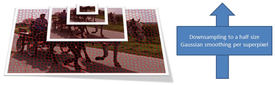
Bottom-up saliency model generation using superpixels
Patrik Polatsek, Wanda Benesova
Slovenska Technicka Univ. (Slovakia)
Abstract. Prediction of human visual attention is more and more frequently applicable in computer graphics, image processing, humancomputer interaction and computer vision. Human attention is influenced by various bottom-up stimuli such as colour, intensity and orientation as well as top-down stimuli related to our memory. Saliency models implement bottom-up factors of visual attention and represent the conspicuousness of a given environment using a saliency map. In general, visual attention processing consists of identification of individual features and their subsequent combination to perceive whole objects. Standard hierarchical saliency methods do not respect the shape of objects and model the saliency as the pixel-by-pixel difference between the centre and its surround.
The aim of our work is to improve the saliency prediction using a superpixel-based approach whose regions should correspond to objects borders. In this paper we propose a novel saliency method that combines a hierarchical processing of visual features and a superpixel-based segmentation. The proposed method is compared with existing saliency models and evaluated on a publicly available dataset.
Paper will be available in 2015:Â
P. Polatsek and W. Benesova, “Bottom-up saliency model generation using superpixels,†in Proceedings of the Spring Conference on Computer Graphics 2015.
Accelerated gSLIC for Superpixel Generation used in Object Segmentation
Robert Birkus
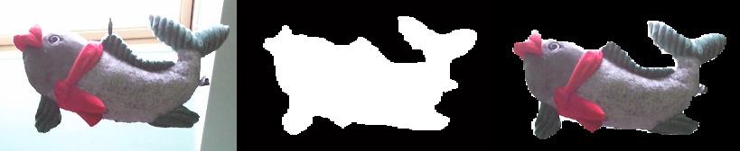
Abstract. The goal of our work is to create a robust object segmentation method which is based on superpixels and will be able to run in real-time applications.
The SLIC algorithm proposed by Achanta et al. [1] is a superpixel segmentation algorithm based on k-means clustering, which efficiently generates superpixels. It seems to be a good trade-off between the time consumption and robustness. Important advancement towards the real time applications using superpixels has been proposed by the authors of the gSLIC – a modified SLIC implementation on the GPU (Graphics Processing Unit) [2].
In this paper, we present a significant acceleration of this superpixel segmentation algorithm gSLIC implemented for the GPU. A different strategy of the implementation on the GPU speeds up the calculation time twice and more over the presented GPU implementation. This implementation can work in real-time even for high resolution images. We also present our method for merging of similar superpixels. This method uses an adaptive decision procedure for merging of superpixels. Accelerated gSLIC is the first part of this proposed object segmentation method.
References
[1] R. Achanta, A. Shaji, K. Smith, A. Lucchi, P. Fua, and S. Susstrunk. Slic superpixels. Technical report, Ecole Polytechnique Fedralede Lausanne , Report No. EPFL-REPORT-149300, 2010.
[2] C. Y. Ren and I. Reid. gSLIC: a real-time implementation of SLIC superpixel segmentation. Technical report, University of Oxford, Department of Engineering, Technical Report (2011)., 2011.
3D local descriptors used in methods of visual 3D object recognition
Marek Jakab, Wanda Benesova
Slovenska Technicka Univ. (Slovakia)
Abstract. In this paper, we propose an enhanced method of 3D object description and recognition based on local descriptors using RGB image and depth information (D) acquired by Kinect sensor. Our main contribution is focused on an extension of the SIFT feature vector by the 3D information derived from the depth map (SIFT-D). We also propose a novel local depth descriptor (DD) that includes a 3D description of the key point neighborhood. Thus defined the 3D descriptor can then enter the decision-making process. Two different approaches have been proposed, tested and evaluated in this paper. First approach deals with the object recognition system using the original SIFT descriptor in combination with our novel proposed 3D descriptor, where the proposed 3D descriptor is responsible for the pre-selection of the objects. Second approach demonstrates the object recognition using an extension of the SIFT feature vector by the local depth description. In this paper, we present the results of two experiments for the evaluation of the proposed depth descriptors. The results show an improvement in accuracy of the recognition system that includes the 3D local description compared with the same system without the 3D local description. Our experimental system of object recognition is working near real-time.
Keywords: local descriptor, depth descriptor, SIFT, segmentation, Kinect v2, 3D object recognition
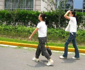
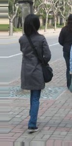
This project focuses on preprocessing of training images for pedestrian detection. The goal is to train a model of a pedestrian detection. Histogram of oriented gradients HOG has been used as descriptor of image features. Support vector machine SVM has been used to train the model.
Example:
Input image
There are several ways to cut train example from source:
using simple bounding rectangle
adding “padding†around simple bounding rectangle
preserve given aspect ratio
using only upper half of pedestrian body
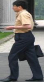
At first, the simple bounding rectangle around pedestrian has been determined. Annotation of training dataset can be used if it is available. In this case a segmentation annotation in form of image mask has been used. Bounding box has been created from image mask using contours (if multiple contours for pedestrian has been found, they were merged to one).);
Each input image has been re-scaled to fit the window size.
1.) Image, which had been cut using simple bounding rectangle, has been resized to fit aspect ratio of descriptor window.
2.) In the next approach the simple bounding rectangle has been enlarged to enrich descriptor vector with background information. Padding of fixed size has been added to each side of image. When the new rectangle exceeded the borders of source image, the source image has been enlarged by replication of marginal rows and columns.
if (params.add_padding)
// Apply padding around patches, handle borders of image by replication
{
	l -= horizontal_padding_size;
	if (l < 0)
	{
		int addition_size = -l;
		copyMakeBorder(timg, timg, 0, 0, addition_size, 0, BORDER_REPLICATE);
		l = 0;
		r += addition_size;
	}
	t -= vertical_padding_size;
	if (t < 0)
	{
		int addition_size = -t;
		copyMakeBorder(timg, timg, addition_size, 0, 0, 0, BORDER_REPLICATE);
		t = 0;
		b += addition_size;
	}
	r += horizontal_padding_size;
	if (r > = timg.size().width)
	{
		int addition_size = r - timg.size().width + 1;
		copyMakeBorder(timg, timg, 0, 0, 0, addition_size, BORDER_REPLICATE);
	}
	b += vertical_padding_size;
	if (b > = timg.size().height)
	{
		int addition_size = b - timg.size().height + 1;
		copyMakeBorder(timg, timg, 0, addition_size, 0, 0, BORDER_REPLICATE);
	}
	allBoundBoxesPadding[i] = Rect(Point(l, t), Point(r, b));
}
3. In the next approach the aspect ratio of descriptor window has been preserved while creating the cutting bounding rectangle (so pedestrian were not deformed). In this case the only necessary padding has been added.
4. In the last approach only the half of pedestrian body has been used.
int hb = t + ((b - t) / 2);
allBoundBoxes[i] = Rect(Point(l, t), Point(r, hb));
NG rng(12345);
static const int MAX_TRIES = 10;
int examples = 0;
int tries = 0;
int rightBoundary = img.size().width - params.neg_example_width / 2;
int leftBoundary = params.neg_example_width / 2;
int topBoundary = params.neg_example_height / 2;
int bottomBoundary = img.size().height - params.neg_example_height / 2;
while (examples < params.negatives_per_image && tries < MAX_TRIES)
{
	int x = rng.uniform(leftBoundary, rightBoundary);
	int y = rng.uniform(topBoundary, bottomBoundary);
	bool inBoundingBoxes = false;
	for (std::vector::iterator it = allBoundBoxes.begin();
		it != allBoundBoxes.end();
		it++)
	{
		if (it->contains(Point(x, y)))
		{
			inBoundingBoxes = true;
			break;
		}
	}
	if (inBoundingBoxes == false) {
		Rect rct = Rect(Point((x - params.neg_example_width / 2), (y - params.neg_example_height / 2)), Point((x + params.neg_example_width / 2), (y + params.neg_example_height / 2)));
		boost::filesystem::path file_neg = (params.negatives_target_dir_path / img_path.stem()).string() + "_" + std::to_string(examples) + img_path.extension().string();
		imwrite(file_neg.string(), img(rct));
		examples++;
	}
	tries++;
}
SVM model has been learned using Matlab function fitcsvm(). The single descriptor vector has been computed:
ay = SVMmodel.Alpha .* SVMmodel.SupportVectorLabels;
sv = transpose(SVMmodel.SupportVectors);
single = sv*ay;
% Append bias
single = vertcat(single, SVMmodel.Bias);
% Save vector to file
dlmwrite(model_file, single,'delimiter','\n');
Single descriptor vector has been loaded and set
( hog.setSVMDetector(descriptor_vector) ) in detection algorithm which used the OpenCV function hog.detectMultiScale() to detect occurrences on multiple scale within whole image.
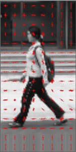
HOG visualization
As a part of project, the HOG descriptor visualization has been implemented. See algorithm bellow. Orientations and magnitudes of gradients are visualized by lines at each position (cell). In first part of algorithm all values from normalization over neighbor blocks at given position has been merged together. Descriptor vector of size 9×4 for one position has yielded vector of size 9.
void visualize_HOG(std::string file_path, cv::Size win_size = cv::Size(64, 128), int
	visualization_scale = 4)
{
	using namespace cv;
	Mat img = imread(file_path, CV_LOAD_IMAGE_GRAYSCALE);
	// resize image (size must be multiple of block size)
	resize(img, img, win_size);
	HOGDescriptor hog(win_size, Size(16, 16), Size(8, 8), Size(8, 8), 9);
	vector descriptors;
	hog.compute(img, descriptors, Size(0, 0), Size(0, 0));
	size_t cell_cols = hog.winSize.width / hog.cellSize.width;
	size_t cell_rows = hog.winSize.height / hog.cellSize.height;
	size_t bins = hog.nbins;
	// block has size: 2*2 cell
	size_t block_rows = cell_rows - 1;
	size_t block_cols = cell_cols - 1;
	size_t block_cell_cols = hog.blockSize.width / hog.cellSize.width;
	size_t block_cell_rows = hog.blockSize.height / hog.cellSize.height;
	size_t binspercellcol = block_cell_rows * bins;
	size_t binsperblock = block_cell_cols * binspercellcol;
	size_t binsperblockcol = block_rows * binsperblock;
	struct DescriptorSum
	{
		vector bin_values;
		int components = 0;
		DescriptorSum(int bins)
		{
			bin_values = vector(bins, 0.0f);
		}
	};
	vector average_descriptors = vector(cell_cols, vector(cell_rows, DescriptorSum(bins)));
	// iterate over block columns
	for (size_t col = 0; col < block_cols; col++)
	{
		// iterate over block rows
		for (size_t row = 0; row < block_rows; row++)
		{
			// iterate over cell columns of block
			for (size_t cell_col = 0; cell_col < block_cell_cols; cell_col++)
			{
				// iterate over cell rows of block
				for (size_t cell_row = 0; cell_row < block_cell_rows; cell_row++)
				{
					// iterate over bins of cell
					for (size_t bin = 0; bin < bins; bin++)
					{
						average_descriptors[col + cell_col][row + cell_row].bin_values[bin] += descriptors[(col*binsperblockcol) + (row*binsperblock) + (cell_col*binspercellcol) + (cell_row*bins) + (bin)];
					}
					average_descriptors[col + cell_col][row + cell_row].components++;
				}
			}
		}
	}
	resize(img, img, Size(hog.winSize.width * visualization_scale, hog.winSize.height * visualization_scale));
	cvtColor(img, img, CV_GRAY2RGB);
	Scalar drawing_color(0, 0, 255);
	float line_scale = 2.f;
	int cell_half_width = hog.cellSize.width / 2;
	int cell_half_height = hog.cellSize.height / 2;
	double rad_per_bin = M_PI / bins;
	double rad_per_halfbin = rad_per_bin / 2;
	int max_line_length = hog.cellSize.width;
	// iterate over columns
	for (size_t col = 0; col < cell_cols; col++)
	{
		// iterate over cells in column
		for (size_t row = 0; row < cell_rows; row++)
		{
			// iterate over orientation bins
			for (size_t bin = 0; bin < bins; bin++)
			{
				float actual_bin_strength = average_descriptors[col][row].bin_values[bin] / average_descriptors[col][row].components;
				// draw lines
				if (actual_bin_strength == 0)
					continue;
				int length = static_cast(actual_bin_strength * max_line_length * visualization_scale * line_scale);
				double angle = bin * rad_per_bin + rad_per_halfbin + (M_PI / 2.f);
				double yrange = sin(angle) * length;
				double xrange = cos(angle) * length;
				Point cell_center;
				cell_center.x = (col * hog.cellSize.width + cell_half_width) * visualization_scale;
				cell_center.y = (row * hog.cellSize.height + cell_half_height) * visualization_scale;
				Point start;
				start.x = cell_center.x + static_cast(xrange / 2);
				start.y = cell_center.y + static_cast(yrange / 2);
				Point end;
				end.x = cell_center.x - static_cast(xrange / 2);
				end.y = cell_center.y - static_cast(yrange / 2);
				line(img, start, end, drawing_color);
			}
		}
	}
	char* window = "HOG visualization";
	cv::namedWindow(window, CV_WINDOW_AUTOSIZE);
	cv::imshow(window, img);
	while (true)
	{
		int c;
		c = waitKey(20);
		if ((char)c == 32)
		{
			break;
		}
	}
}
Cultural and Educational Grant Agency MÅ VVaÅ SR (KEGA) : Integration of visual information studies and creation of comprehensive multi-medial study materials.
Visual detection and object recognition are the main challenges of computer vision. Detection and recognition systems can be used in surveillance, medicine, robotics or augmented reality applications. Image pre-processing is used for removing unwanted image effects like signal noise; edge detection, blur removal, etc. in order to get images suitable for further processing.
Next step in the pipeline is the extraction of relevant and discriminative features for classification. The role of the classification is to assign the object to the correct class of objects. The last part of the book deals with color theory describing colorimetric functions and color spaces for computer vision. Lastly, visual perception theory, including eye tracking and visual saliency detection methods is described.
The book is intended not only for students, but also for the broad technical audience.
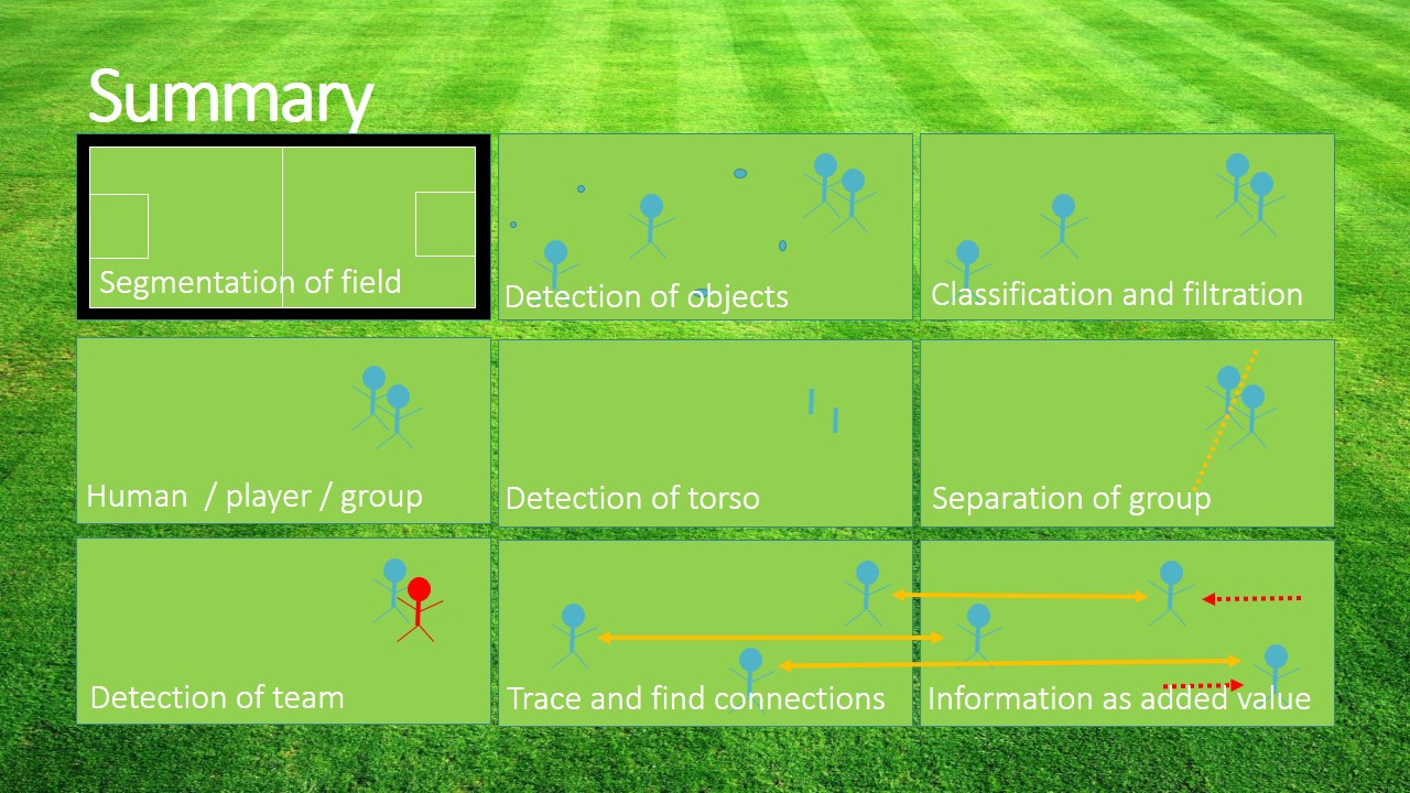
Try detect objects (players, soccer ball, referees, goal keeper) in soccer match. Detect their position, movement and show picked object in ROI area. More info in a presentation and description document.
T. D’Orazio, M.Leo, N. Mosca, P.Spagnolo, P.L.Mazzeo A Semi-Automatic System for Ground Truth Generation of Soccer Video Sequences in the Proceeding of the 6th IEEE International Conference on Advanced Video and Signal Surveillance, Genoa, Italy September 2-4 2009
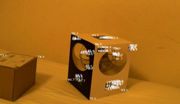
This example presents straightforward process to determine depth of points (sparse depth map) from stereo image pair using stereo reconstruction. Example is implemented in Python 2.
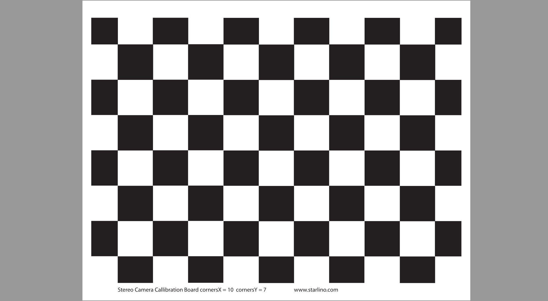
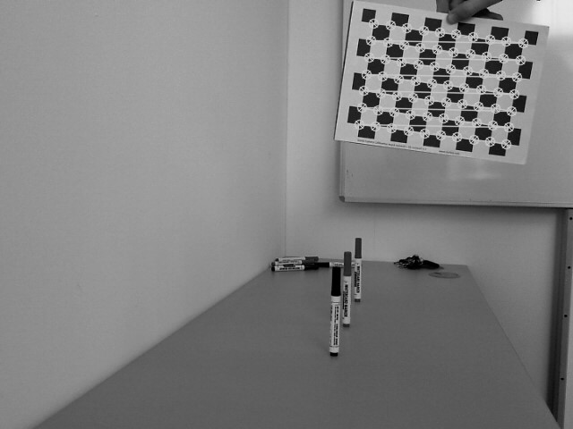
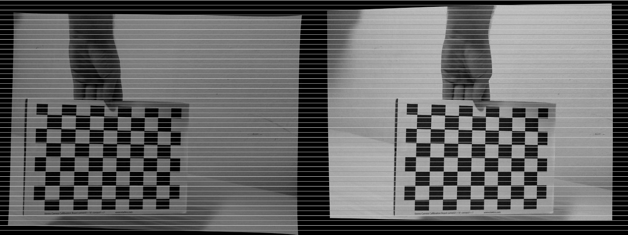
Stereo calibration process
We need to obtain multiple stereo pairs with chessboard shown on both images.
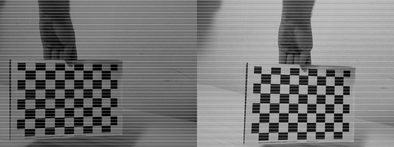
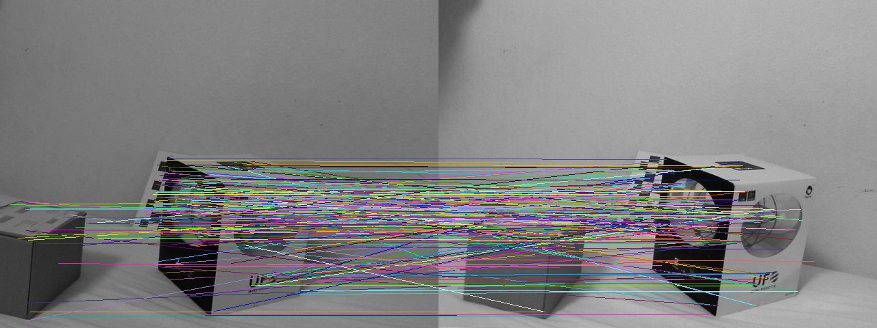
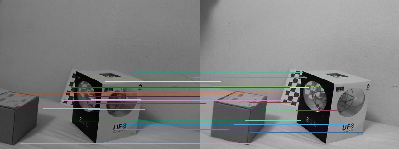
Standard object matching: keypoint detection (Harris, SIFT, SURF,…), descriptor extractor (SIFT, SURF) and matching (Flann, brute force,…). Matches are filtered for same line coordinates to remove mismatches.
detector = cv2.FeatureDetector_create("HARRIS")
extractor = cv2.DescriptorExtractor_create("SIFT")
matcher = cv2.DescriptorMatcher_create("BruteForce")

for pair in pairs:
    left_kp = detector.detect(pair.left_img_remap)
    right_kp = detector.detect(pair.right_img_remap)
    l_kp, l_d = extractor.compute(left_img_remap, left_kp)
    r_kp, r_d = extractor.compute(right_img_remap, right_kp)
    matches = matcher.match(l_d, r_d)
    sel_matches = [m for m in matches if abs(l_kp[m.queryIdx].pt[1] - r_kp[m.trainIdx].pt[1]) < 3]
Raw keypoint matches on cropped rectified imagesSame line matches
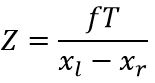
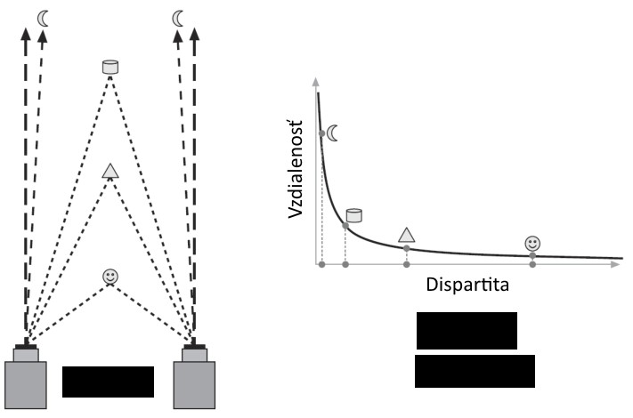
Triangulation
How do we get depth of point? Dispartity is difference of x coordinate of the same keypoint in both images. Closer points have greater dispartity and far points have almost zero dispartity. Depth can be defined as:
Where:
f – focal length
T – baseline – distance of cameras
x1, x2 – x coordinated of same keypoint
Z – depth of point
for m in sel_matches:
        left_pt = l_kp[m.queryIdx].pt
        right_pt = r_kp[m.trainIdx].pt
        dispartity = abs(left_pt[0] - right_pt[0])
        z = triangulation_constant / dispartity
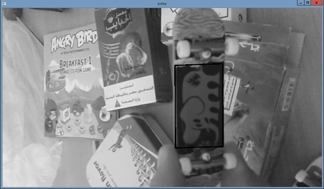
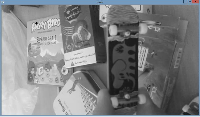
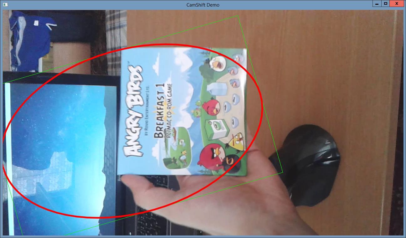
In our work we focus on basics of motion analysis and object tracking. We compare MeanShift (non-parametric, finds an object on a back projection image) versus CamShift (continuously adaptive mean shift, finds an object center, size, and orientation) algorithms and effectively utilize them to perform simple object tracking. In case these algorithms fail to track the desired object or the object travels out of window scope, we try to find another object to track. To achieve this, we use a background subtractor based on a Gaussian Mixture Background / Foreground Segmentation Algorithm to identify the next possible object to track. There are two suitable implementations of this algorithm in OpenCV – BackgroundSubtractorMOG and BackgroundSubtractorMOG2. We also compare performance of both these implementations.
Used functions:Â calcBackProject, calcHist, CamShift, cvtColor, inRange, meanShift, moments, normalize
Solution
Initialize tracking window:
Set tracking window near frame center
Track object utilizing MeanShift / CamShift
Calculate HSV histogram of region of interest (ROI) and track
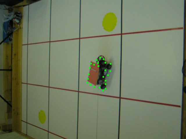
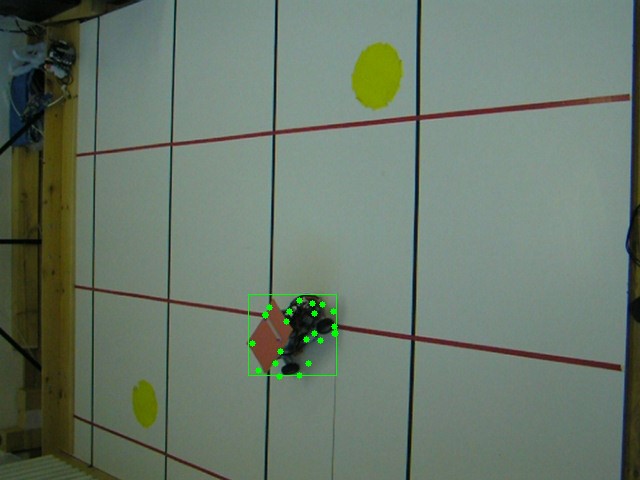
As seen on Fig. 1, MeanShift (left) operates with fixed size tracking windows which can not be rotated. On the contrary, CamShift (right) utilizes the full potential of dynamic size rotated rectangles. Working with CamShift yielded significantly better tracking results in general. On the other hand we recommend to use MeanShift when the object is in constant distance from the camera and moves without rotation (or is represented by a circle), in such case MeanShift performs faster than CamShift and produces sufficient results without any rotation or size change noise.
Fig. 1: MeanShift vs. CamShift.
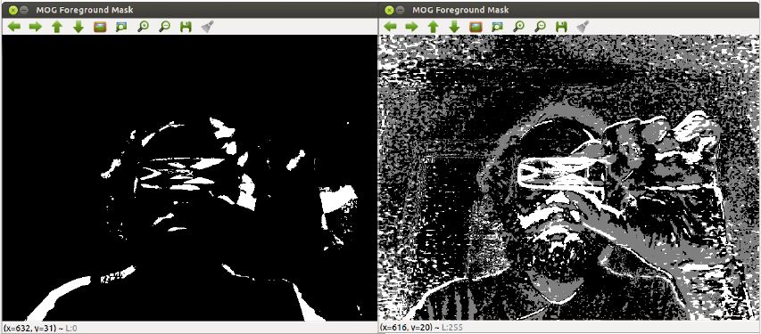
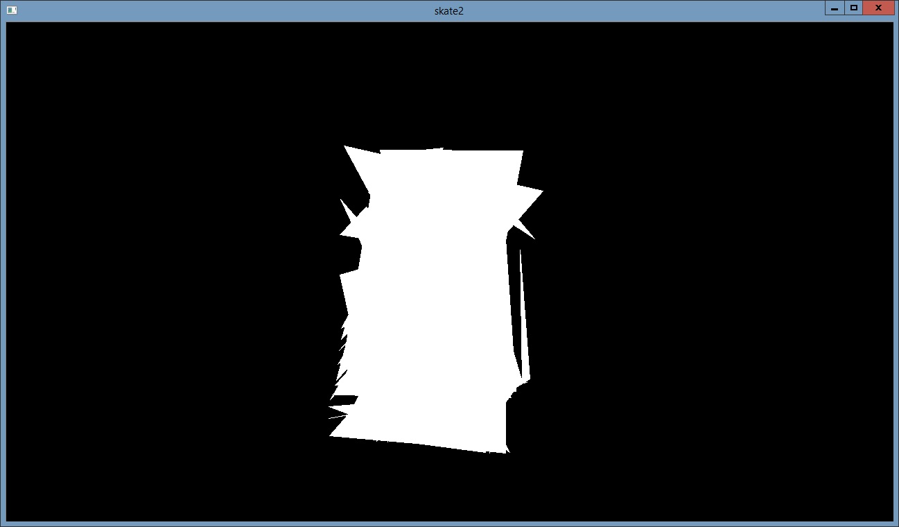
Comparison of BackgroundSubtractorMOG and BackgroundSubtractorMOG2 is depicted on Fig. 2. MOG approach is simpler than MOG2 as it considers only binary masks whereas MOG2 operates on a full gray scale masks. Experiments shown that in our specific case MOG performed better as it yielded less information noise than MOG2. MOG2 will probably produce better results than MOG when utilized more effectively than in out initial approach (simple centeroid from mask extraction).
Fig. 2: MOG vs. MOG2.
Summary
In this project explored the possibilities of simple object tracking via OpenCV APIs utilizing various algorithms such as MeanShift and CamShift, Background Extractor MOG and MOG2, which we also compared. Our solution performs relatively well, but we can certainly improve it by fine tuning histogram calculation, MOG, and other parameters. Other improvements can be done in MOG usage, as now the objects are only recognized by finding MOG mask centeroids. This also calls to better tracking window initialization process.
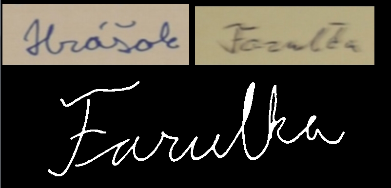
Main purpose of this project was to recognise signatures. For this purpose we used descriptor from the bottom of the signature. Then we used Mahalanobis distance to identify signatures.
Image preprocessing
We have worked with 2 sets of signatures and each of them had about 200 pictures of signatures. Examples of those signatures are below.
Input signatures
The signatures had different quality. So we decided to find skeleton of them.
Mat skel(tmp_image.size(), CV_8UC1, Scalar(0));
Mat tmp(tmp_image.size(), CV_8UC1);

Mat structElem = getStructuringElement(MORPH_CROSS, Size(3, 3));

do
{
	morphologyEx(tmp_image, tmp, MORPH_OPEN, structElem);
	bitwise_not(tmp, tmp);
	bitwise_and(tmp_image, tmp, tmp);
	bitwise_or(skel, tmp, skel);
	erode(tmp_image, tmp_image, structElem);

	double max;
	minMaxLoc(tmp_image, 0, &max);
	done = (max == 0);
} while (!done);
Skeleton of the signature
Then we decided to find contours and filter them according to their size to remove the noise.
vector<vector<Point>> contours;
vector<Vec4i> hierarchy;

findContours(image, contours, hierarchy, CV_RETR_TREE, CV_CHAIN_APPROX_SIMPLE);

Mat drawing = Mat::zeros(image.size(), CV_8UC1);
for (int i = 0; i< contours.size(); i++){
	if (contours[i].size() < 10.0) continue;
	Scalar color = Scalar(255);
	drawContours(drawing, contours, i, color, CV_FILLED, 8, hierarchy);
}
The result of image preprocessed like this can be seen below. This picture has very thick lines so we decided to add contour image and skeleton image together.
Contour image
For purpose of adding 2 images together we used logical function AND.
bitwise_and(newImage, skeleton, contours);
The result of this process was signature with thin line with no noise.
Creating descriptors
To create descriptors we used bottom line of the signature. To lower the factor of length of signature we always divided signature to 25 similar pieces. Space between these pieces was calculated dynamically. The descriptor was gathered as maximum of white point position in each of 25 division points.
To reduce the factor that signature is written in some angle we transformed the points to lower positions. To do so we gathered points in 10° range from lowest point. Then we calculated average of these points. Then we used linear regression to add coefficient to all points. Linear regression was made using maximal point and average of the other points.
Descriptor we created had counted with different lengths of signatures and different angles of signatures. So the last step was to normalise the height. To do so we subtracted minimum point of the signature from all points and then we divided all points with maximum from descriptor.
Learning phase
We created 2 sets of descriptors each with 180 examples. From these descriptors we created 2 objects of class Signature.
class Signature
{
	std::string name; //signature name
	cv::Mat centorid; //centorid created from learning set
	cv::Mat covarMat; //covariance matrix created form lenrning set
};
To recognition of the signatures we wanted to use Mahalanobis distance method. To do so we needed centroid for our data set and inverse covariance matrix. We calculated those using functions:
In code above the variable samples is representing the matrix of all samples.
Testing
After we created inverse covariance matrix and centroid we could start testing. Testing of the signature was creating its descriptor using same steps as when creating descriptors in testing set. Then we could call function to calculate Mahalanobis distance.
Using this algorithm we were able to identify some of the signatures. But the algorithm is very sensitive to changes in image quality and number of items in training set.
This example shows how to separate and track moving object using OpenCV. First, the background of the video is being calculated and moving objects detected, then it is filtered and tracked.
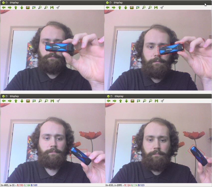
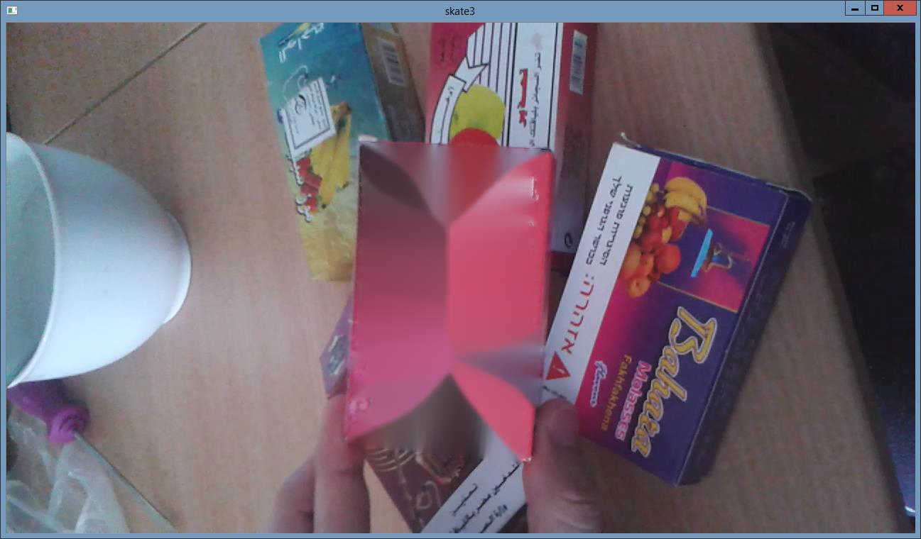
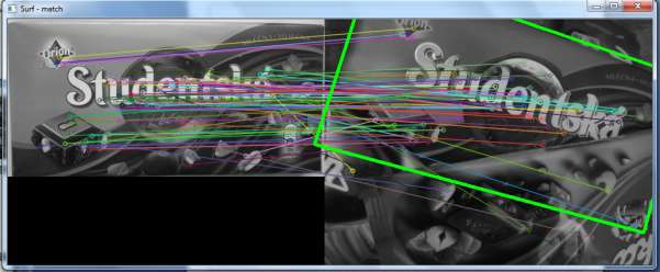
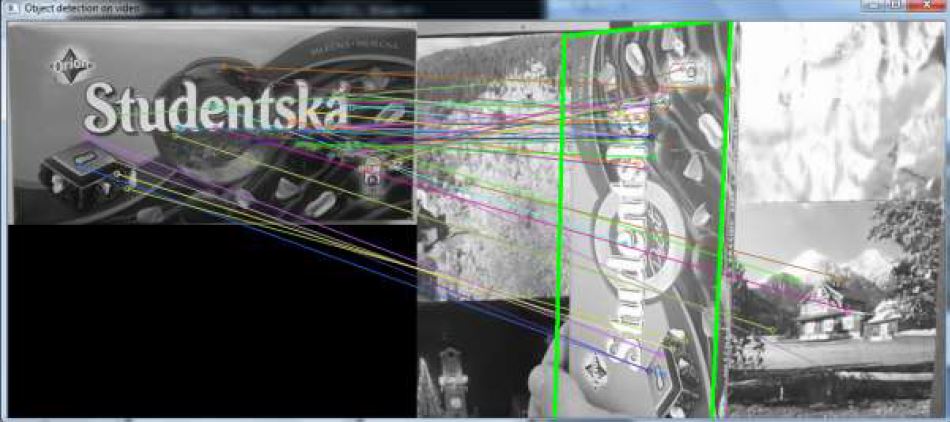
In our project we focus on simple object recognition, then tracking this recognized object and finally we try to delete this object from video. By object recognition we used local features-based methods. We compare SIFT and SURF methods for detection and description. By RANSAC algorithm we compute the homography. In case these algorithms successfully find the object we create a mask where recognized object was white area and the rest was black. By object tracking we compared the two approaches. The first approach is based on calculating optical flow using the iterative Lucas-Kanade method with pyramids. The second approach is based on camshift tracking algorithm. For deleting the object from video we focus to using algorithm based on restoring the selected region in an image using the region neighborhood.
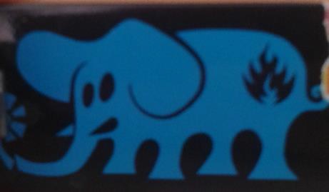
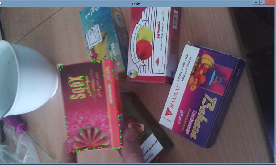
The project shows detection of chocolate cover from input image or frame of video. For each video or image may be chosen various combinations of detector with descriptor. For matching object of chocolate cover with input frame or image automatically is used FlannBasedMatcher or BruteForceMatcher. It depends on the chosen SurfDescriptorExtractor or FREAK algorithm.