Ján Kvak

Abstract. In this paper we propose a way to create a visual words using binary descriptor and to cluster and classify them from input images using Sparse Distributed Memory with genetic algorithms. SDM could be used as a new approach to refine clustering of binary descriptors and in the same algorithm create a classifier capable of quick clustering of this particular input data. In the second section we propose to add a binary tree to this classifier to be able to quickly classify input data to predefined classes.
Introduction
The image recognition and classification is becoming an area of huge interest lately. However the reliable and fast algorithm that could recognize any object in input scene as fast humans are able to do, is still something to be discovered. For now the algorithms are always tradeoffs between reliability, speed and number of classes that can be recognized.
As the object recognition capability is something, that we want to approximate, we can study the principles of human thinking and object categorization, to use them in image recognition algorithms. Because the human language and word recognition is well studied area, the principles of recognizing human speech can be used in object recognition [1]. We can treat object classes as words that can represent clusters of descriptors, which are good for recognition.

In [2] authors provide a chart representing general algorithm of creation and usage of bag of words. This algorithm is illustrated in Figure 1. Their approach to creating and using visual words is to extract local descriptors from a set of input images divided to N classes. Then they clustered this set of local descriptors using K-means algorithm. Clustering provided them with “codebook†of words, in which the words were centers of clusters. Then each image can be represented as a
“bag of visual wordsâ€. These bags of words can be trained into classifier. Authors used hierarchical Bayesian models. In different work [3] Naive Bayes classifier and SVM were used for this purpose.
In these works, SIFT local descriptor was used to describe keypoints found in input images. SIFT has become de-facto standard in local descriptors area and all new ones are compared to its capabilities. One of major drawbacks of this local descriptor is, that it is relatively slow to compute, so for a practical use, the approximations like SURF has emerged. Among the new local descriptors that are regularly compared to SIFT, are binary feature descriptors like ORB, BRISK and FREAK. These descriptors are represented with vector of bits, so they can be compared and stored efficiently and quickly. In this work, we will use the latest one FREAK, which capabilities are compared to SIFT in [4].
We can now use the fact, that all local features are represented as binary vectors. Clustering and classifying now takes place in Hamming space, because we can compare these features using Hamming distance. For this purpose we propose the use of Sparse Distributed Memory (SDM) augmented with genetic algorithms also called genetic memory[5].
Genetic memory
In [5] genetic memory was used to predict weather. Weather samples were converted to vectors of bits and trained to memory. It is a variation of Kanerva’s Sparse Distributed Memory (SDM) augmented with Holland’s genetic algorithms. SDM takes advantage of sparse distribution of input data in high-dimensional binary address space. It can be represented as a three – layer neural network with an extremely large number of hidden nodes in middle layer (1,000,000 +) [5]
SDM is an associative memory, which purpose is to store data, and retrieve them, if address we call is sufficiently close to the address, at which data were stored. If the address we call is sufficiently close to the address, at which data were stored, the associative memory, in this case SDM , should return data with less noise, than the noise in the original address. [6]

Figure 2 shows a structure of SDM. We can see that it consists mainly from two parts – location addresses and n-bit counters. It has constant radius that describes maximum distance to location address, in which this address is still selected. Then, we have reference addresses, which denote the classes, we want to train. The fact worth noting is that the number of reference addresses is much bigger than the number of location addresses.
When training, we need training data that belong to each one of reference addresses. In Sparse Distributed Memory, the location addresses, which distance in Hamming space is smaller than radius of memory, are selected. For one reference address it is usually more location addresses. Then training data, belonging to reference address are used to alter the counters in selected location addresses. If that particular bit in training data is 1, counter is incremented, in the case of 0, counter is decremented.
Reading from memory means, that we need input address that we want to correct. Output of this procedure should be the reference address that this input belongs to. This input is compared to each one of location addresses and the ones, closer than radius to the input address, are selected. Counters from selected addresses are column wise summed. The sum is then converted to bit vector that is the reference address.
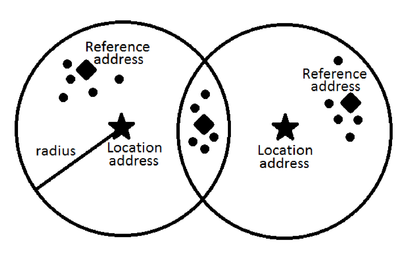
In Figure 3. we can see visualization of Sparse Dispersed Memory working principles. Marked by a star, there are two location addresses. Around them, we have an area, denoted by radius, which show the addresses that belong to that particular location. Reference addresses are marked by a diamond. Dots mark data that belong to that particular reference address.
From this visualization, we can see, that to represent three classes (three reference addresses) we need only two location addresses.
The problem is how to choose location addresses, to represent well the data that we want to classify. This is why authors of [5] used Holland’s genetic algorithm to choose the location addresses, that would be best to represent the input data classes.
In the beginning, the location addresses are filled with random bits. After training each of the input classes, we compute fitness function for all of the location addresses. Fitness function states, how good is the location at representing input data. Then two of the location addresses with the best rating according to fitness function are chosen to create a new address, which can then replace the address with lowest rating. Genetic combination is made at one or more crossover points.

Using this algorithm, locations after multiple generations should evolve towards the ones that are best to represent input reference addresses and corresponding input data. Other consequence is, that after training, the reference address on the output of memory is also moving towards the address more representing input data. The output of counters effectively average[7] the data given in input, so the reference address is in the “middle†of classified data.

In the Figure 5 we can see the reference address before training and after training of data. So training of genetic memory have two important results – it creates location addresses, that can represent input data and they refine reference addresses from input, so they can be better recognized by this particular SDM.
Forming of codebook
We propose to use genetic memory to create and train visual words. First we must roughly choose the reference addresses that can be than used to train SDM. That can be done using clustering algorithm like K-means. Then after they are trained to SDM and multiple generations of genetic refinement are used to create the best possible locations, to classify this particular codebook. After this is done, when we try to read from trained SDM, we need to present it with input bit vector obtained from the classified point in image. However this kind of memory after fixed number of steps, which is lower than the number of visual words, gives us only a bit vector, which is a reference address. But for the purpose of visual words, we need to get the number of the reference address, not the complete vector. Observing the SDM, we can say, that always the one combination of local addresses belong to one class which can be denoted by a number.
To this end, we could use simple binary tree. Every level of the tree should belong to one of the location addresses. The leaves of the tree will be marked with numbers of reference addresses. As we can see from Figure 6 the input data vector that we need to assign to one of the classes, (one of the visual words) is compared to all of location addresses. After each comparing, we move to the next node of the binary tree according to the result of comparing. In this case we move to the right, if Hamming distance of input vector from location address is smaller than radius, if not, we move to the left. That means, that to assign vector to one of the classes (visual words) we still need only fixed number of steps, that is number of location addresses. This can be a significant save of time, if the number of visual words is large, because number of location addresses << number of visual words.

Experiments
We propose an experiment to evaluate this hypothesis. In this experiment, we use the collection of input images, to create a visual word codebook and then to classify them. For this purpose we want to use Caltech 101 image dataset. For the purpose of describing the image points, we can use binary descriptors FREAK and ORB. From this dataset, we can create the codebook using only SDM with genetic algorithms, then using K-means clustering algorithm and refining in SDM and for comparison, using only K-means. Then, after creating the codebook, we compare speed and accuracy of classification of visual words in SDM with classification in Naive Bayes and SVM classifiers.
Preliminary experiments with SDM with genetic algorithms show, that one of the problems with this type of memory is choosing the right fitness function. If the location addresses are set randomly, there is high probability, that without right fitness function, only same two best addresses will be always chosen and the children of this genetic crossover will be positioned only next to small part of reference addresses, thus not effectively describing all of input data. This happens, when the parents for crossover are chosen absolutely[5]. Second option is to choose them probabilistically [5]. The best members are chosen randomly, but proportionally to their fitness function. Other problem is, that in [5] authors did not describe complete genetic algorithm, that requires mutations as well as genetic crossovers. Experiments on smaller data showed, that it is necessary to include genetic mutations to algorithm.

As we can see from Figure 7, if the optimal location address contains bits (the ones in the grey part), that are not present in best location addresses from parent generation no type of crossover can create desired result.
Conclusions
We proposed a way of creating visual codebook and to classify image patches described by binary vectors to visual words using Spares Distributed Memory with genetic algorithms. This genetic memory is capable of classifying great number of classes, while maintaining constant number of steps in the process of recognizing. It is equal to a neural network with great number of neurons and it is designed to operate on great number of sparse distributed data in Hamming space. Using genetic memory, we can refine the visual words gained from dataset and, in the same time create classifier, adapted to recognize visual words from that same dataset. Augmenting genetic memory with binary tree, we can get numbers of visual words, instead of their binary vectors, without increasing the complexity and computing time of the algorithm.
References
[1] J. Sivic and A. Zisserman, “Video Google: a text retrieval approach to object matching in videos,†Proceedings Ninth IEEE International Conference on Computer Vision, no. Iccv, pp. 1470–1477 vol.2, 2003.
[2] P. Perona, “A Bayesian Hierarchical Model for Learning Natural Scene Categories,†2005 IEEE Computer Society Conference on Computer Vision and Pattern Recognition (CVPR’05), vol. 2, pp. 524–531.
[3] G. Csurka, C. R. Dance, L. Fan, J. Willamowski, C. Bray, and D. Maupertuis, “Visual Categorization with Bags of Keypoints,†In Workshop on statistical learning in computer vision ECCV, vol. 1, p. 22, 2004.
[4] A. Alahi, R. Ortiz, and P. Vandergheynst, “FREAK: Fast Retina Keypoint,†2012 IEEE Conference on Computer Vision and Pattern Recognition, pp. 510–517, Jun. 2012.
[5] D. Rogers, “Weather Prediction Using Genetic Memory,†1990.
[6] D. Rogers, “Kanerva’s sparse distributed memory: An associative memory algorithm wellsuited to the Connection Machine,†1988.
[7] D. Rogers, “Statistical prediction with Kanervas Sparse Distributed Memory,†1989.