This post provides an example of image filtration and editing in the frequency domain. Practical methods of image spectrum conversion and Gaussian mask creation are described. The sample application is written in C++ using the OpenCV 2.x API. The full source code is also attached.
Image data transformation into the frequency domain
In frequency domain we can analyze the spectrum of signals.  The known Fourier transform is a linear transformation used for the conversion from time (e.g. audio signals in 1 dimension) or spatial (e.g. image in 2 dimensions) domain into the frequency domain. By the definition of Furier trasform is given, that the spectral  data are complex numbers in general.OpenCV library include functions for calculation of Discrete Fourier Transform of an input image into a complex matrix – spectrum.
The next sample function shows a possibility to use the filtration in frequency domain for the enhancement of the image. Optimal DFT size was achieved by the method “zero padding”.
Note: Resolution of complex output can be increased by multiplying M and N variables with a constant.
[c language=”c++”]
Mat computeDFT(Mat image) {
Mat padded;
int m = getOptimalDFTSize(image.rows);
int n = getOptimalDFTSize(image.cols);
// create output image of optimal size
copyMakeBorder(image, padded, 0, m – image.rows, 0, n – image.cols, BORDER_CONSTANT, Scalar::all(0));
// copy the source image, on the border add zero values
Mat planes[] = { Mat_< float> (padded), Mat::zeros(padded.size(), CV_32F) };
// create a complex matrix
Mat complex;
merge(planes, 2, complex);
dft(complex, complex, DFT_COMPLEX_OUTPUT);Â // fourier transform
return complex;
}
[/c]
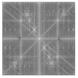
Once the complex matrix is generated, the visualization of spectrum can be done by  the OpenCV operation  magnitude (which is per-element matrix operation) and then by the conversion into the logarithmic scale for proper display.
Note: shift() function does the rearrangement of quadrants using SetROI() and CopyTo() functions of OpenCV API. See the full source code for more details.
[c language=”c++”]
void updateMag(Mat complex) {
Mat magI;
Mat planes[] = {
Mat::zeros(complex.size(), CV_32F),
Mat::zeros(complex.size(), CV_32F)
};
split(complex, planes); // planes[0] = Re(DFT(I)), planes[1] = Im(DFT(I))
magnitude(planes[0], planes[1], magI); // sqrt(Re(DFT(I))^2 + Im(DFT(I))^2)
// switch to logarithmic scale: log(1 + magnitude)
magI += Scalar::all(1);
log(magI, magI);
shift(magI); // rearrage quadrants
// Transform the magnitude matrix into a viewable image (float values 0-1)
normalize(magI, magI, 1, 0, NORM_INF);
imshow("spectrum", magI);
}
[/c]
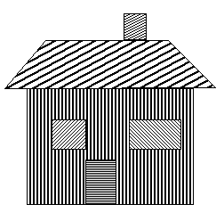
Processing
This project was designed as an interactive tool which can clear somelocal extremes in spectrum by multiplying it with a Gauss filter. OpenCV framework provides functions to handle mouse clicks and input trackballs, please see the full source code for more details.
First of all we need to create a Gaussian mask, if we working with in frequency domain we need to consider that, the spectrum is symmetric, so the mask is also need to mirrored by image center.
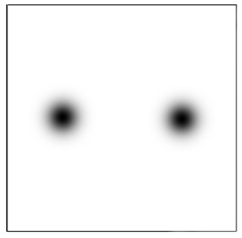
For processing image in frequency domain, we would like use the Gaussian mask as a complex matrix and multiply it with the original image’s spectrum.
[c language=”c++”]
Mat mask = createGausFilterMask(complex.size(), x, y, kernel_size, true, true);
shift(mask); // rearrange quadrants of mask
Mat planes[] = {
Mat::zeros(complex.size(), CV_32F),
Mat::zeros(complex.size(), CV_32F)
};
Mat kernel_spec;
planes[0] = mask; // real
planes[1] = mask; // imaginar
merge(planes, 2, kernel_spec);
mulSpectrums(complex, kernel_spec, complex, DFT_ROWS); //only DFT_ROWS flag is accepted
[/c]
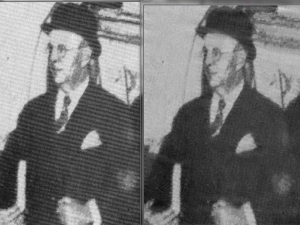
Results
The backward transformation from the frequency domain is handled by using inverse DFT.
[c language=”c++”]
void updateResult(Mat complex)
{
Mat result;
idft(complex, result);
// equivalent to:
// dft(complex, result, DFT_INVERSE + DFT_SCALE);
Mat planes[] = {
Mat::zeros(complex.size(), CV_32F),
Mat::zeros(complex.size(), CV_32F)
};
split(result, planes); // planes[0] = Re(DFT(I)), planes[1] = Im(DFT(I))
magnitude(planes[0], planes[1], result); // sqrt(Re(DFT(I))^2 + Im(DFT(I))^2)
normalize(result, result, 0, 1, NORM_MINMAX);
imshow("result", result);
}
[/c]
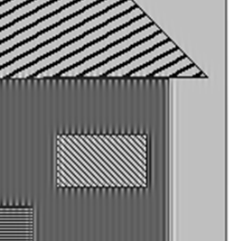
Practical samples