Posted on

Bag of Words Classifier

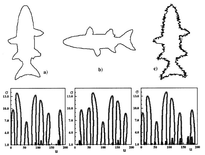
In computer vision and object recognition, we have three main areas – object classification, detection and segmentation. Classification task deals only with assigning an image to a class (for example bicycle, dog, cactus, etc…), detection task moreover deals with detecting the position of the object in an image and segmentation task deals with finding the detailed contours of the object. Bag of words is a method which belongs to classification problem.

Algorithm steps

  1. Find key points in images using Harris detector.
    Ptr<DescriptorMatcher> matcher = DescriptorMatcher::create("FlannBased");
    Ptr<DescriptorExtractor> extractor = DescriptorExtractor::create("SIFT");
    Ptr<FeatureDetector> detector = FeatureDetector::create("HARRIS");
    
  2. Extract SIFT local feature vectors from the set of images.
    // Extract SIFT local feature vectors from set of images
    extractTrainingVocabulary("data/train", extractor, detector, bowTrainer);
    
  3. Put all the local feature vectors into a single set.
    vector<Mat> descriptors = bowTrainer.getDescriptors();
    
  4. Apply a k-means clustering algorithm over the set of local feature vectors in order to find centroid coordinates. This set of centroids will be the vocabulary.
    cout << "Clustering " << count << " features" << endl;
    Mat dictionary = bowTrainer.cluster();
    
    cout << "dictionary.rows == " << dictionary.rows << ", dictionary.cols == " << dictionary.cols << endl;
    
  5. Compute the histogram that counts how many times each centroid occurred in each image. To compute the histogram find the nearest centroid for each local feature vector.
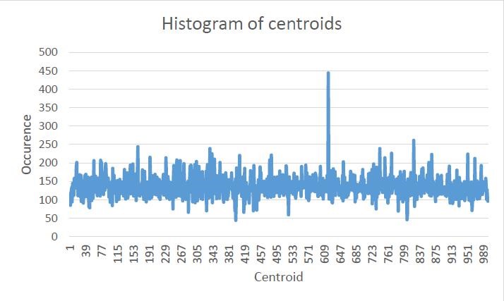
Histogram

We trained our model on 240 different images from 3 different classes – bonsai, Buddha and porcupine. We then computed the following histogram which counts how many times each centroid occurred in each image. To find the values of the histogram we had to compare the distances of each local feature vector with each centroid and centroid with least difference to local feature vector has incremented in histogram. We used 1000 cluster centers.

Posted on

Concrete Analysis

Description

In this work, we have detected a metallic wires on slide concrete. Metal parts are distributed randomly. It may happen that the positions of two adjacent wires or also cutting the wires along the length. Some wires are due to bad picture almost invisible. The images we applied filters from the library OpeCV and we have created an application that can recognize about 90% of the wires.

Input

Processing

  1. Create marker of image
    cv::erode(_grayScale, marker,
        cv::getStructuringElement(cv::MORPH_ELLIPSE,
        cv::Size(20, 20), cv::Point(-1,-1)), cv::Point(-1,-1), 2,
        cv::borderInterpolate(1, 15, cv::BORDER_ISOLATED));
    ImReconstruct(&amp;(IplImage)marker, &amp;(IplImage)_grayScale);
    

  2. Substraction grayscale image and marker image
    grayScale = _grayScale - marker;
    

  3. Use some morphological operation and get contours
    // Closing, erode, treshold
    cv::findContours(grayScale.clone(), contours, CV_RETR_TREE, CV_CHAIN_APPROX_SIMPLE, cv::Point(0,0) );
    
  4. Detailed analysis of the use of wires, in specific cases

  5. Final output

Posted on

Dominant Orientation Templates

Description

Dominant orientation templates (DOT) is a method for real-time object detection, which works well for detection of untextured objects and is related to method Histogram of oriented gradients. DOT is neither based on statistical learning of object’s shapes nor on feature point detection, but it uses real-time Template Matching recognition with locally most dominant orientations from HoG.

OpenCV function used

cvCaptureFromAVI, cvtColor

The process

  1. Computation of gradients for each pixel in template and input image
    1. Provided by convolution kernel
    2. For each pixel
    3. Gradient is defined by magnitude and direction
    4. 0-180° instead of 0-360° range
    5. Directions can be discretized from 0-180° into bins (e.g. 9 bins by 20° )
    for (int r=0;r<=area.rows-region_size;r+=region_size)
    {
        for (int s=0;s<=area.cols-region_size;s+=region_size)
        {
            int mag=gradienty_template.gradient[i][j].magnitude;
            n0=histogram_group(gradienty_template.gradient[i][j].direction);
            if (mag>min_magnitude)
                template_hist.hist_matrix[hx][hy].bins[n0]+=mag;
        }
    }
    
  2. Dividing pixels into regions

    for (int r=0;r<=area.rows-region_size;r+=region_size)
        // moving in the picture with step size of 7 or 9
    
  3. Computing most dominant gradient orientations for each region

    if (template_hist.hist_matrix[i][j].bins[k]>max) //now only the most dominant
    {
        if  (template_hist.hist_matrix[i][j].bins[k]>min_magnitude)
        {
            max=template_hist.hist_matrix[i][j].bins[k];
            max_index=k;
        }
    }
    
  4. Template matching and comparing of most dominant orientations.
  5. Evaluating comparison.

Posted on

Eye Blinking Detection

Description

The main purpose of this work is to detect eyes and recognize when are open and when close. To execute this purpose we must use video camera or video file with person face.

Eye Detection

To detect eye blinking we need to recognize face and eyes on image. For this intention we use Viola Jones algorithm which detect this features and bounded it with rectangles.

Because this algorithm is performance consuming, we use tracking which is more faster. We use Good Features to Track algorithm which return set of points suitable to track, and then with Lucas-Kanade tracker algorithm we track it on every frame.

// track points
calcOpticalFlowPyrLK(prevGray, gray, features, cornersB, status, error, Size(31, 31), 1000);

if(!calculateIntegralHOG(gray(rectangleFace)))
    text = "CLOSED";

There is problem with points which is not precisely targeted to next frame, so we remove them from set of tracking points. When number of points is not enough to track, we repeat eye detection method again.

Eye Blinking Detection

To detect if eyes are open or close we use HOG descriptor which return array of floats representing lines orientation. Because HOG descriptor is usable only on images with specific resolution, we use sliding window with this resolution which covers our image.

cv::gpu::HOGDescriptor gpu_hog(win_size, Size(16, 16), Size(8, 8), Size(8, 8), 9, 0.8, 0.00015, true);

// calculate HOG for every window
GpuMat gpuMat;
gpuMat.upload(cropped);
GpuMat descriptors;
gpu_hog.getDescriptors(gpuMat, win_size, descriptors);
Mat descriptorMat = Mat(descriptors);

In next step we take array of floats returned from HOG descriptor and transform it to histogram. We notice, that when eye is closed the local maximum of this histogram is much lower than local maximum of opened eye, so we define the value which separate opened and closed eye.

Because we use sliding window, we average all this local maxims and based on returned value, we decide if specified area contains open or close eyes.

Posted on

Dices Result Recognition

Description

The goal of this project is to implement algorithm that finds dots on dices. Motivation was idea / question how to create home-made random number generator? We can throw dices and our application will be able to recognize summary value on dices.

This program uses fitEllipse() function to find dots on dices. The basics steps are as follows:

Process

  1. Open video stream
    CvCapture* capture = cvCaptureFromCAM( CV_CAP_ANY );
    
  2. For the whole stream we create single frame
    IplImage* frame = cvQueryFrame( capture );
    
  3. Invert color
  4. Use adaptive threshold
    adaptiveThreshold(image, bimage, 255, ADAPTIVE_THRESH_GAUSSIAN_C, CV_THRESH_BINARY, 15, -10);
    
  5. We can use morphological operations (dilatation, erosion) to expand/minimize contours
  6. To find circles we use following:
    Mat pointsf;
    Mat(contours[i]).convertTo(pointsf, CV_32F);
    RotatedRect box = fitEllipse(pointsf);
    
  7. If difference between box.size.width and box.size.height is lower than treshold, we consider ellipse as circle.
  8. At this point we have a lot of “circles”. An experimenting helped us to determine, which circle in the picture is real point on dice. Based on size of real dices points we can isolate only real dices points.

Example of process

Original grayscale image
Inverted colors
Adaptive threshold – 255 (invert)
Histogram of points size
Lots of custom settings
RESULT!

Using custom settings we are able to improve results in specific situations.

findContours(bimage, contours, CV_RETR_LIST, CV_CHAIN_APPROX_NONE);

Vector<pair<RotatedRect*, int>> vec, finalVec;
Mat cimage = Mat::zeros(bimage.size(), CV_8UC3);
int i;
int w, h, wAhThr, angleThr, centerThr;
int  hwDifferenceThreshold, histThreshold;						
centerThr = settCenterThr;
wAhThr = settwAhThr;
hwDifferenceThreshold = settHWdifferenceThr;
histThreshold = settHistogramThr;

for(i = 0; i < contours.size(); i++)
{
	size_t count = contours[i].size();
	if( count > 50 || count  < 6)
	      continue;

	Mat pointsf;
	Mat(contours[i]).convertTo(pointsf, CV_32F);
	RotatedRect box = fitEllipse(pointsf);

	w = box.size.width;
	h = box.size.height;

	int hwDifference = abs(h - w);
	if (hwDifference > hwDifferenceThreshold)
	      continue;

	if (w < wAhThr || h < wAhThr)
	      continue;

	vec.push_back(pair<RotatedRect*, int>(new RotatedRect(box), i));
}

int asdf = vec.size();
Vector<pair<RotatedRect* ,int>>::iterator it ,iend, it2;
int MAXHIST = 200;
int* histVals = new int[MAXHIST];
for (int i = 0; i < MAXHIST; i++)
	histVals[i] = 0;

int histIter = 0;
RotatedRect * box;
RotatedRect * box2;
int maxWidth = 0;
int distanceOfCenters;
for (it = vec.begin(), iend = vec.end(); it != iend; it++)
{
	box = (it->first);
	for (it2 = it + 1; it2 != iend; it2++)
	{
		box2 = (it2->first);
		distanceOfCenters = (int)std::sqrt((box->center.x - box2->center.x) * (box->center.x - box2->center.x) + (box->center.y - box2->center.y)  * (box->center.y - box2->center.y));
		if (distanceOfCenters < centerThr)
		{
			if (box->size.width > box2->size.width)
				it2->second = -1;
			else
				it->second = -1;
			break;
		}

	}
}
Posted on

CSS – Curvature Scale Space in OpenCV

Description

The goal of this project is to implement algorithm that creates curvature scale space (CSS) image of given shape using OpenCV library. “The CSS image consists of several arch-shape contours representing the inflection points of the shape as it is smoothed. The maxima of these contours are used to represent a shape. The CSS representation is robust with respect to scale, noise and change in orientation.”[1]

CSS representations for various curve modifications [1]

Process

  1. Find contour coordinates of given shape
  2. findContours(im, contours, CV_RETR_LIST, CV_CHAIN_APPROX_NONE );
    

    Following steps are repeated with increased sigma until there are no zero-crossing points:

  3. Gaussian kernel is the base for upcoming steps:
    transpose(getGaussianKernel(width, sigma, CV_64FC1), G);
    
  4. Curve evolution can be computed by convolution of contour points with Gaussian kernel. Smoothed contour is not needed for CSS computation; it is used only to visualize the process:

    filter2D(X, Xsmooth, X.depth(), G);
    filter2D(Y, Ysmooth, Y.depth(), G);
    

    Curve evolution with increasing sigma [2]
  5. To compute 1st and 2nd derivation of contour points, Gaussian kernel derivations will be needed:
    Sobel(G, dG, G.depth(), 1, 0, 3);
    Sobel(G, ddG, G.depth(), 2, 0, 3);
    
  6. Convolution of contour points using derivatives of Gaussian kernel. According to OpenCV documentation: filter2D does actually computes correlation, not the convolution. That is, the kernel is not mirrored around the anchor point. If you need a real convolution, flip the kernel using flip() and set the new anchor to (kernel.cols – anchor.x – 1, kernel.rows – anchor.y – 1) :
    flip(dg, dg, 0);
    flip(ddg, ddg, 0);
    Point anchor(dg.cols - fwhm -1, dg.rows - 0 - 1);
    filter2D(X, dX, X.depth(), dG, anchor);
    filter2D(Y, dY, Y.depth(), dG, anchor);
    filter2D(X, ddX, X.depth(), ddG, anchor);
    filter2D(Y, ddY, Y.depth(), ddG, anchor);
    
  7. Finally, we calculate the curvature and find zero crossings:

    Curvature and inflection points of curve smoothed with sigma=16
  8. Zero-crossing points are plotted to the final CSS image. X-axis represents position of point on the curve; Y-axis represents the value of sigma:
    Final CSS image with zero-crossing points for all sigmas

Practical Applications

  • Finding similar shapes  (Used as shape descriptor in MPEG-7 standard)
  • Corner detection
Example of cornes detection

References

[1] Sadegh Abbasi, Farzin Mokhtarian, Josef Kittler: Curvature Scale Space Image in Shape Similarity Retrieval. Multimedia Syst. 7(6): 467-476 (1999)

[2] Farzin Mokhtarian, Alan K. Mackworth: A Theory of Multiscale, Curvature-Based Shape Representation for Planar Curves. IEEE Trans. Pattern Anal. Mach. Intell. 14(8): 789-805 (1992)

Posted on

Detection and removal of circular artifacts from photographs

Description

Reflecting flashlight from dust, snowflakes or raindrops can produce irritating circular artifacts. For its detecting and removing we propose process, where we use improved circle detection besides using houghCircles function. For removing detected artifacts we use morphological reduction.

Functions used

adaptiveThreshold, Canny, HoughCircles, findContours, fitEllipse, ImReconstruct

Process

Greyscale input image with circular artifacts.
Output image.

Limitation: Minimal circle size (15px )- Maximal circle size(30px)

  1. Preprocessing – Adaptive threshold
    medianBlur()
    adaptiveThreshold()
    OutputImg := InputImg + FilteredImg
    
  2. Detection with HoughCircles
    Canny()
    GaussianBlur()
    HoughCircles()
    Accept/ignore circles (based on size)
    
  3. Detection with Morphological reconstruction and contour analysis
    mask := InputImg
    marker := InputImg – degreeOfMorphreduct
    marker := inv(marker)
    morphologicalReconstruction(marker, mask)
    differenceImg := marker2 – marker1
    differenceImg := medianBlur(differenceImg)
    differenceImg := threshold(differenceImg)
    contour[] = findContours (differenceImg)
    ellipse[i] := fitEllipse(contour[i])
    accept/ignore circles (based on size and ellipse axes)
    draw white ellipse[i]
    draw black contour[i]
    crop Regions Of Interest
    opening(regionOfInterest[i])
    if countNonZero(regionOfInterest[i]) > threshold then accept; else ignore;
    
  4. Result

Posted on

Convolutional neural networks

Description

Convolutional Neural Networks(CNNs) are multi-layered neural networks with standard hidden layers and with at least one convolutional layer. They are suitable for visual processing because they exploit the tolopogy of inputs.

Because we are interested in more general structures of networks and layers, the CNN is implemented with automatic differentiation (AD) in mind. This means that one has to provide only the implementation of forward pass of any structure. It is important to note that AD is based on certainly different principle as finite differences. The important difference of AD is that it yields precise results.

Architecture

The architecture of convolutional networks is shown in figure 1. Convolutional layers are located right after inputs. After each convolutional layer the process of subsampling is performed. By subsampling we improve translational invariance and significantly reduce complexity. After convolutional layers, standard fully connected hidden layers are used. These are then mapped to desired outputs.

Architecture of convolutional networks.

When the signal passes into standard hidden layer, it is no longer meaningful to pass it again into another convolutional layers. However it can be meaningful to have heterogeneous layers consisting of convolutional and also standard units.

Experiments

Note that it is meaningful for input to be two-dimensional. We have used CNN for handwritten digits recognition of US Postal Service.

  • 2,5% human error rate
  • 2,0% best error rate: combination of multiple classifiers
  • 4,7% best achievement of our CNN

We note, that CNNs are sensitive to parameter settings including number and size of convolutional kernels. However, when properly set, CNNs perform well. We can see an example output of convolutional layers at figure 2.

Example of features extracted in the first convolutional layer.
Posted on

Hand Tracking and Gesture Recognition Using Echo State Neural Networks

Peter Fillo

recognizerFilloHand Tracking and Gesture Recognition Using Echo State Neural Networks. Tracking an object in a video sequence is a complex problem which presents one of the fundamental task of image processing. One of the many use cases is controlling using hand gestures in Human-Computer Interaction. This paper introduces real-time hand recognition and tracking in video sequence with a classification of performed hand gestures. Hand recognition is based on foreground segmentation and skin region detection. Attributes of hand movements are being recorded and used as an input to a echo state neural network which performs hand gesture classification. Work presents proposed tracking algorithm and first results of gesture recognition.