Posted on

CSS – Curvature Scale Space in OpenCV

Description

The goal of this project is to implement algorithm that creates curvature scale space (CSS) image of given shape using OpenCV library. “The CSS image consists of several arch-shape contours representing the inflection points of the shape as it is smoothed. The maxima of these contours are used to represent a shape. The CSS representation is robust with respect to scale, noise and change in orientation.”[1]

CSS representations for various curve modifications [1]

Process

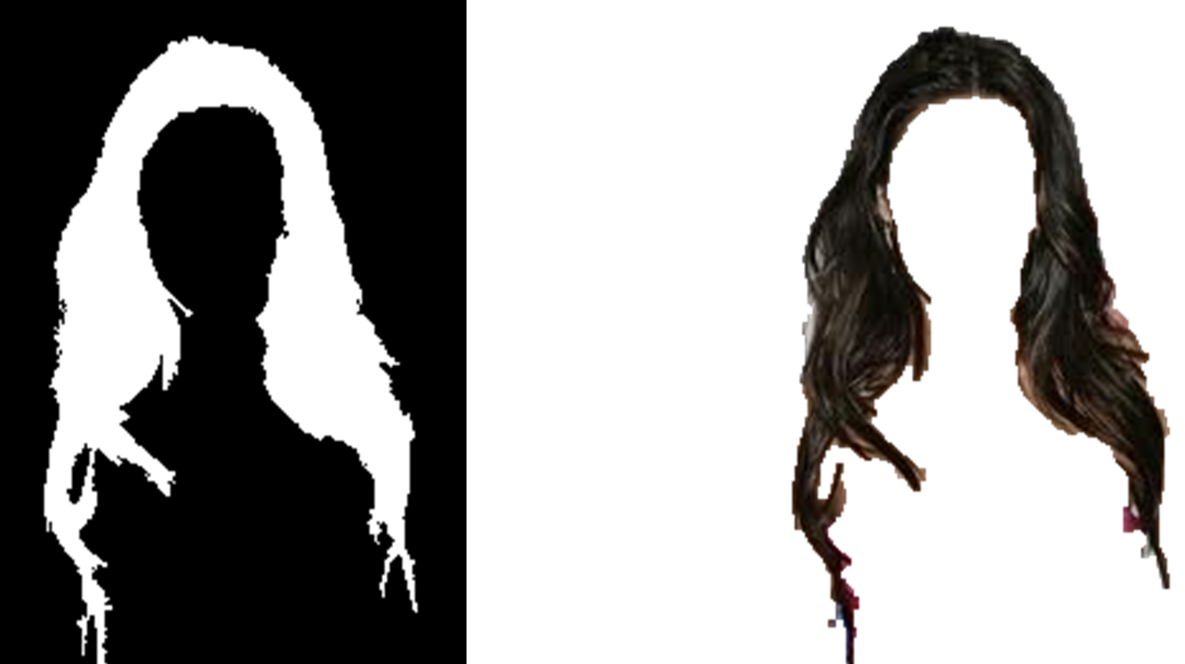
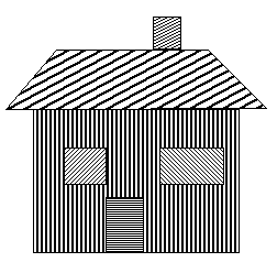
  1. Find contour coordinates of given shape
  2. findContours(im, contours, CV_RETR_LIST, CV_CHAIN_APPROX_NONE );
    

    Following steps are repeated with increased sigma until there are no zero-crossing points:

  3. Gaussian kernel is the base for upcoming steps:
    transpose(getGaussianKernel(width, sigma, CV_64FC1), G);
    
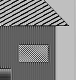
  4. Curve evolution can be computed by convolution of contour points with Gaussian kernel. Smoothed contour is not needed for CSS computation; it is used only to visualize the process:

    filter2D(X, Xsmooth, X.depth(), G);
    filter2D(Y, Ysmooth, Y.depth(), G);
    

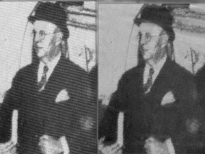
    Curve evolution with increasing sigma [2]
  5. To compute 1st and 2nd derivation of contour points, Gaussian kernel derivations will be needed:
    Sobel(G, dG, G.depth(), 1, 0, 3);
    Sobel(G, ddG, G.depth(), 2, 0, 3);
    
  6. Convolution of contour points using derivatives of Gaussian kernel. According to OpenCV documentation: filter2D does actually computes correlation, not the convolution. That is, the kernel is not mirrored around the anchor point. If you need a real convolution, flip the kernel using flip() and set the new anchor to (kernel.cols – anchor.x – 1, kernel.rows – anchor.y – 1) :
    flip(dg, dg, 0);
    flip(ddg, ddg, 0);
    Point anchor(dg.cols - fwhm -1, dg.rows - 0 - 1);
    filter2D(X, dX, X.depth(), dG, anchor);
    filter2D(Y, dY, Y.depth(), dG, anchor);
    filter2D(X, ddX, X.depth(), ddG, anchor);
    filter2D(Y, ddY, Y.depth(), ddG, anchor);
    
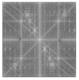
  7. Finally, we calculate the curvature and find zero crossings:

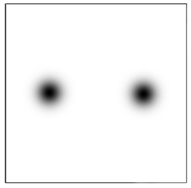
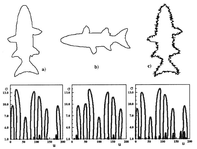
    Curvature and inflection points of curve smoothed with sigma=16
  8. Zero-crossing points are plotted to the final CSS image. X-axis represents position of point on the curve; Y-axis represents the value of sigma:
    Final CSS image with zero-crossing points for all sigmas

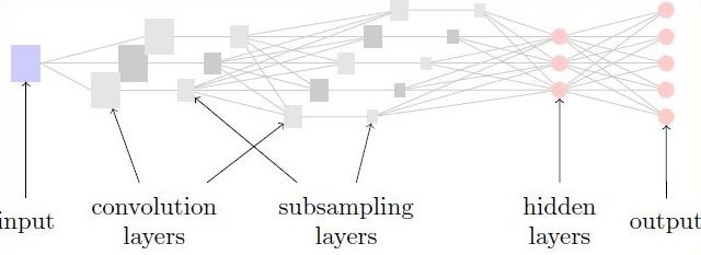
Practical Applications

  • Finding similar shapes  (Used as shape descriptor in MPEG-7 standard)
  • Corner detection
Example of cornes detection

References

[1] Sadegh Abbasi, Farzin Mokhtarian, Josef Kittler: Curvature Scale Space Image in Shape Similarity Retrieval. Multimedia Syst. 7(6): 467-476 (1999)

[2] Farzin Mokhtarian, Alan K. Mackworth: A Theory of Multiscale, Curvature-Based Shape Representation for Planar Curves. IEEE Trans. Pattern Anal. Mach. Intell. 14(8): 789-805 (1992)

Posted on

Hair segmentation

Description

The project shows hair segmentation from photos. Important thing is to have an appropriate input image, where background and hair color must be different. Algorithm uses Mean Shift segmentation to segment input image into regions. Best regions are selected to be in the final image.

OpenCV function used

cvHaarDetectObjects, cvSplit, cvCalcHist, cvGetMinMaxHistValue, cvInRangeS

The process

  1. appropriate image selection
  2. face detection
  3. face segmentation (optional)
  4. Mean Shift image segmentation
  5. first region selection
  6. expansion of the first region
  7. final hair segmentation from image

Sample

Input image
From left: haar face detection, colors reduction, mean shift segmentation.
Initial hair region selection.
Left: neighboring regions, right: adding neighboring regions.
Left: mask created, right: Hair segmentation final image.
Posted on

Detection and removal of circular artifacts from photographs

Description

Reflecting flashlight from dust, snowflakes or raindrops can produce irritating circular artifacts. For its detecting and removing we propose process, where we use improved circle detection besides using houghCircles function. For removing detected artifacts we use morphological reduction.

Functions used

adaptiveThreshold, Canny, HoughCircles, findContours, fitEllipse, ImReconstruct

Process

Greyscale input image with circular artifacts.
Output image.

Limitation: Minimal circle size (15px )- Maximal circle size(30px)

  1. Preprocessing – Adaptive threshold
    medianBlur()
    adaptiveThreshold()
    OutputImg := InputImg + FilteredImg
    
  2. Detection with HoughCircles
    Canny()
    GaussianBlur()
    HoughCircles()
    Accept/ignore circles (based on size)
    
  3. Detection with Morphological reconstruction and contour analysis
    mask := InputImg
    marker := InputImg – degreeOfMorphreduct
    marker := inv(marker)
    morphologicalReconstruction(marker, mask)
    differenceImg := marker2 – marker1
    differenceImg := medianBlur(differenceImg)
    differenceImg := threshold(differenceImg)
    contour[] = findContours (differenceImg)
    ellipse[i] := fitEllipse(contour[i])
    accept/ignore circles (based on size and ellipse axes)
    draw white ellipse[i]
    draw black contour[i]
    crop Regions Of Interest
    opening(regionOfInterest[i])
    if countNonZero(regionOfInterest[i]) > threshold then accept; else ignore;
    
  4. Result

Posted on

Convolutional neural networks

Description

Convolutional Neural Networks(CNNs) are multi-layered neural networks with standard hidden layers and with at least one convolutional layer. They are suitable for visual processing because they exploit the tolopogy of inputs.

Because we are interested in more general structures of networks and layers, the CNN is implemented with automatic differentiation (AD) in mind. This means that one has to provide only the implementation of forward pass of any structure. It is important to note that AD is based on certainly different principle as finite differences. The important difference of AD is that it yields precise results.

Architecture

The architecture of convolutional networks is shown in figure 1. Convolutional layers are located right after inputs. After each convolutional layer the process of subsampling is performed. By subsampling we improve translational invariance and significantly reduce complexity. After convolutional layers, standard fully connected hidden layers are used. These are then mapped to desired outputs.

Architecture of convolutional networks.

When the signal passes into standard hidden layer, it is no longer meaningful to pass it again into another convolutional layers. However it can be meaningful to have heterogeneous layers consisting of convolutional and also standard units.

Experiments

Note that it is meaningful for input to be two-dimensional. We have used CNN for handwritten digits recognition of US Postal Service.

  • 2,5% human error rate
  • 2,0% best error rate: combination of multiple classifiers
  • 4,7% best achievement of our CNN

We note, that CNNs are sensitive to parameter settings including number and size of convolutional kernels. However, when properly set, CNNs perform well. We can see an example output of convolutional layers at figure 2.

Example of features extracted in the first convolutional layer.
Posted on

Frequency domain filtration

This post provides an example of image filtration and editing in the frequency domain. Practical methods of image spectrum conversion and Gaussian mask creation are described. The sample application is written in C++ using the OpenCV 2.x API. The full source code is also attached.

Image data transformation into the frequency domain

In frequency domain we can analyze the spectrum of signals.  The known Fourier transform is a linear transformation used for the conversion from time (e.g. audio signals in 1 dimension) or spatial (e.g. image in 2 dimensions) domain into the frequency domain. By the definition of Furier trasform is given, that the spectral  data are complex numbers in general.OpenCV library include functions for calculation of Discrete Fourier Transform of an input image into a complex matrix – spectrum.
The next sample function shows a possibility to use the filtration in frequency domain for the enhancement of the image. Optimal DFT size was achieved by the method “zero padding”.
Note: Resolution of complex output can be increased by multiplying M and N variables with a constant.

Mat computeDFT(Mat image) {
	Mat padded;
	int m = getOptimalDFTSize(image.rows);
	int n = getOptimalDFTSize(image.cols);
	// create output image of optimal size
	copyMakeBorder(image, padded, 0, m - image.rows, 0, n - image.cols, BORDER_CONSTANT, Scalar::all(0));
	// copy the source image, on the border add zero values
	Mat planes[] = { Mat_< float> (padded), Mat::zeros(padded.size(), CV_32F) };
	// create a complex matrix
	Mat complex;
	merge(planes, 2, complex);
	dft(complex, complex, DFT_COMPLEX_OUTPUT);  // fourier transform
	return complex;
}

Once the complex matrix is generated, the visualization of spectrum can be done by  the OpenCV operation  magnitude (which is per-element matrix operation) and then by the conversion into the logarithmic scale for proper display.

Note: shift() function does the rearrangement of quadrants using SetROI() and CopyTo() functions of OpenCV API. See the full source code for more details.

void updateMag(Mat complex) {
	Mat magI;
	Mat planes[] = {
		Mat::zeros(complex.size(), CV_32F),
		Mat::zeros(complex.size(), CV_32F)
	};
	split(complex, planes); // planes[0] = Re(DFT(I)), planes[1] = Im(DFT(I))
	magnitude(planes[0], planes[1], magI); // sqrt(Re(DFT(I))^2 + Im(DFT(I))^2)
	// switch to logarithmic scale: log(1 + magnitude)
	magI += Scalar::all(1);
	log(magI, magI);
	shift(magI); // rearrage quadrants
	// Transform the magnitude matrix into a viewable image (float values 0-1)
	normalize(magI, magI, 1, 0, NORM_INF);
	imshow("spectrum", magI);
}

Processing

This project was designed as an interactive tool which can clear somelocal extremes in spectrum by multiplying it with a Gauss filter. OpenCV framework provides functions to handle mouse clicks and input trackballs, please see the full source code for more details.

First of all we need to create a Gaussian mask, if we working with in frequency domain we need to consider that, the spectrum is symmetric, so the mask is also need to mirrored by image center.

A symmetric Gaussian mask

For processing image in frequency domain, we would like use the Gaussian mask as a complex matrix and multiply it with the original image’s spectrum.

Mat mask = createGausFilterMask(complex.size(), x, y, kernel_size, true, true);
shift(mask);  // rearrange quadrants of mask

Mat planes[] = {
	Mat::zeros(complex.size(), CV_32F),
	Mat::zeros(complex.size(), CV_32F)
};
Mat kernel_spec;
planes[0] = mask; // real
planes[1] = mask; // imaginar
merge(planes, 2, kernel_spec);

mulSpectrums(complex, kernel_spec, complex, DFT_ROWS); //only DFT_ROWS flag is accepted

Results

The backward transformation from the frequency domain is handled by using inverse DFT.

void updateResult(Mat complex)
{
	Mat result;
	idft(complex, result);
	// equivalent to:
	// dft(complex, result, DFT_INVERSE + DFT_SCALE);
	Mat planes[] = {
		Mat::zeros(complex.size(), CV_32F),
		Mat::zeros(complex.size(), CV_32F)
	};
	split(result, planes); // planes[0] = Re(DFT(I)), planes[1] = Im(DFT(I))
	magnitude(planes[0], planes[1], result); // sqrt(Re(DFT(I))^2 + Im(DFT(I))^2)
	normalize(result, result, 0, 1, NORM_MINMAX);
	imshow("result", result);
}
Sample result (cropped)

Practical samples

Watch the Sample screen video

Sample 1: digitally transmitted image with periodic noise
Sample 2: scanned postcard

Further reading

Posted on

Frequency domain filtration – source

#include 

using namespace cv;
using namespace std; 

void onMouse( int event, int x, int y, int, void* param);
void updateMag(Mat complex);
void updateResult(Mat complex);

Mat computeDFT(Mat image);
Mat createGausFilterMask(Size mask_size, int x, int y, int ksize, bool normalization, bool invert);
void shift(Mat magI);

int kernel_size = 0;

int main( int argc, char** argv )
{ 

	String file;
	file = " << SAMPLE FILE >>";

	Mat image = imread(file, CV_LOAD_IMAGE_GRAYSCALE);
	namedWindow( "Orginal window", CV_WINDOW_AUTOSIZE  );// Create a window for display.
	imshow( "Orginal window", image );                   // Show our image inside it.

	Mat complex = computeDFT(image);

	namedWindow( "spectrum", CV_WINDOW_AUTOSIZE );
    createTrackbar( "Gausian kernel size", "spectrum", &kernel_size, 255, 0 );
    setMouseCallback( "spectrum", onMouse, &complex);

	updateMag(complex);			// compute magnitude of complex, switch to logarithmic scale and display...
	updateResult(complex);		// do inverse transform and display the result image
	waitKey(0);	

	return 0;
}

void onMouse( int event, int x, int y, int, void* param)
{
    if( event != CV_EVENT_LBUTTONDOWN )
        return;
	// cast *param to use it local
	Mat* p_complex = (Mat*) param;
	Mat complex = *p_complex;

	Mat mask = createGausFilterMask(complex.size(), x, y, kernel_size, true, true);
	// show the kernel
	imshow("gaus-mask", mask);

	shift(mask); 

	Mat planes[] = {Mat::zeros(complex.size(), CV_32F), Mat::zeros(complex.size(), CV_32F)};
	Mat kernel_spec;
	planes[0] = mask; // real
	planes[1] = mask; // imaginar
    merge(planes, 2, kernel_spec);

	mulSpectrums(complex, kernel_spec, complex, DFT_ROWS); // only DFT_ROWS accepted

	updateMag(complex);		// show spectrum
	updateResult(complex);		// do inverse transform

	*p_complex = complex;

	return;
}

void updateResult(Mat complex)
{
	Mat work;
	idft(complex, work);
//	dft(complex, work, DFT_INVERSE + DFT_SCALE);
	Mat planes[] = {Mat::zeros(complex.size(), CV_32F), Mat::zeros(complex.size(), CV_32F)};
	split(work, planes);                // planes[0] = Re(DFT(I)), planes[1] = Im(DFT(I))

	magnitude(planes[0], planes[1], work);	  // === sqrt(Re(DFT(I))^2 + Im(DFT(I))^2)
	normalize(work, work, 0, 1, NORM_MINMAX);
	imshow("result", work);
}

void updateMag(Mat complex )
{

	Mat magI;
	Mat planes[] = {Mat::zeros(complex.size(), CV_32F), Mat::zeros(complex.size(), CV_32F)};
	split(complex, planes);                // planes[0] = Re(DFT(I)), planes[1] = Im(DFT(I))

    magnitude(planes[0], planes[1], magI);    // sqrt(Re(DFT(I))^2 + Im(DFT(I))^2)

	// switch to logarithmic scale: log(1 + magnitude)
	magI += Scalar::all(1);
    log(magI, magI);

	shift(magI);
    normalize(magI, magI, 1, 0, NORM_INF); // Transform the matrix with float values into a
                                              // viewable image form (float between values 0 and 1).
    imshow("spectrum", magI);
}

#include "dft_routines.h";

Mat computeDFT(Mat image) {
	// http://opencv.itseez.com/doc/tutorials/core/discrete_fourier_transform/discrete_fourier_transform.html
	Mat padded;                            //expand input image to optimal size
    int m = getOptimalDFTSize( image.rows );
    int n = getOptimalDFTSize( image.cols ); // on the border add zero values
    copyMakeBorder(image, padded, 0, m - image.rows, 0, n - image.cols, BORDER_CONSTANT, Scalar::all(0));
	Mat planes[] = {Mat_(padded), Mat::zeros(padded.size(), CV_32F)};
	Mat complex;
    merge(planes, 2, complex);         // Add to the expanded another plane with zeros
	dft(complex, complex, DFT_COMPLEX_OUTPUT);  // furier transform
	return complex;
}

Mat createGausFilterMask(Size mask_size, int x, int y, int ksize, bool normalization, bool invert) {
	// Some corrections if out of bounds
	if(x < (ksize / 2)) {
		ksize = x * 2;
	}
	if(y < (ksize / 2)) {
		ksize = y * 2;
	}
	if(mask_size.width - x < ksize / 2 ) {
		ksize = (mask_size.width - x ) * 2;
	}
	if(mask_size.height - y < ksize / 2 ) {
		ksize = (mask_size.height - y) * 2;
	}

	// call openCV gaussian kernel generator
	double sigma = -1;
	Mat kernelX = getGaussianKernel(ksize, sigma, CV_32F);
	Mat kernelY = getGaussianKernel(ksize, sigma, CV_32F);
	// create 2d gaus
	Mat kernel = kernelX * kernelY.t();
	// create empty mask
	Mat mask = Mat::zeros(mask_size, CV_32F);
	Mat maski = Mat::zeros(mask_size, CV_32F);

	// copy kernel to mask on x,y
	Mat pos(mask, Rect(x - ksize / 2, y - ksize / 2, ksize, ksize));
	kernel.copyTo(pos);

	// create mirrored mask
	Mat posi(maski, Rect(( mask_size.width - x) - ksize / 2, (mask_size.height - y) - ksize / 2, ksize, ksize));
	kernel.copyTo(posi);
	// add mirrored to mask
	add(mask, maski, mask);

	// transform mask to range 0..1
	if(normalization) {
		normalize(mask, mask, 0, 1, NORM_MINMAX);
	}

	// invert mask
	if(invert) {
		mask = Mat::ones(mask.size(), CV_32F) - mask;
	}

	return mask;
}

void shift(Mat magI) {

    // crop if it has an odd number of rows or columns
	magI = magI(Rect(0, 0, magI.cols & -2, magI.rows & -2));

	int cx = magI.cols/2;
    int cy = magI.rows/2;

    Mat q0(magI, Rect(0, 0, cx, cy));   // Top-Left - Create a ROI per quadrant
    Mat q1(magI, Rect(cx, 0, cx, cy));  // Top-Right
    Mat q2(magI, Rect(0, cy, cx, cy));  // Bottom-Left
    Mat q3(magI, Rect(cx, cy, cx, cy)); // Bottom-Right

    Mat tmp;                            // swap quadrants (Top-Left with Bottom-Right)
    q0.copyTo(tmp);
    q3.copyTo(q0);
    tmp.copyTo(q3);
    q1.copyTo(tmp);                     // swap quadrant (Top-Right with Bottom-Left)
    q2.copyTo(q1);
    tmp.copyTo(q2);
}
Posted on

Hand Tracking and Gesture Recognition Using Echo State Neural Networks

Peter Fillo

recognizerFilloHand Tracking and Gesture Recognition Using Echo State Neural Networks. Tracking an object in a video sequence is a complex problem which presents one of the fundamental task of image processing. One of the many use cases is controlling using hand gestures in Human-Computer Interaction. This paper introduces real-time hand recognition and tracking in video sequence with a classification of performed hand gestures. Hand recognition is based on foreground segmentation and skin region detection. Attributes of hand movements are being recorded and used as an input to a echo state neural network which performs hand gesture classification. Work presents proposed tracking algorithm and first results of gesture recognition.