Posted on

Detection of cities and buildings in the images

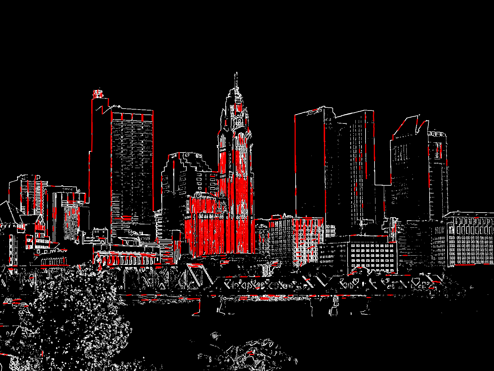
Project is focused on the image detection which major components are cities and buildings. Buildings and cities detection assumes occurence of the edges as implication of the Windows and walls, as well as presence of the sky. Algorithm creates the feature vector with SVM classification algorithm.

Functions used: HoughLinesP, countNonZero, Sobel, threshold, merge, cvtColor, split, CvSVM

The process

  1. Create edge image
    cv::Sobel(intput, grad_x, CV_16S, 1, 0, 3, 1, 0, cv::BORDER_DEFAULT);
    cv::Sobel(intput, grad_y, CV_16S, 0, 1, 3, 1, 0, cv::BORDER_DEFAULT);
    
  2. Find lines in the binary edge image
    cv::HoughLinesP(edgeImage, edgeLines, 1, CV_PI / 180.0, 1, 10, 0);
    
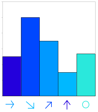
  3. Count numbers of lines in specified tilt
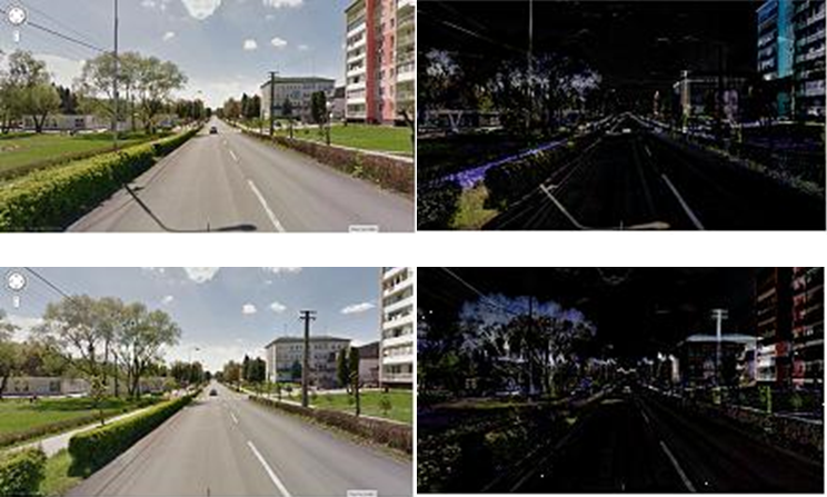
  4. Convert original image to HSV color space and remove saturation and value
    cv::cvtColor(src, hsv, CV_BGR2HSV);
    
  5. Process the image from top to bottom , if pixel is not blue then all pixels under him are not sky
  6. Classification with SVM
    CvSVMParams params;
    params.svm_type  = CvSVM::C_SVC;
    params.kernel_type = CvSVM::LINEAR;
    params.term_crit   = cvTermCriteria(CV_TERMCRIT_ITER, 5000, 1e-5);
    
    float OpencvSVM::predicate(std::vector<float> features)
    {
       std::vector<std::vector<float> > featuresMatrix;
       featuresMatrix.push_back(features);
       cv::Mat featuresMat = createMat(featuresMatrix);
       return SVM.predict(featuresMat);
    }
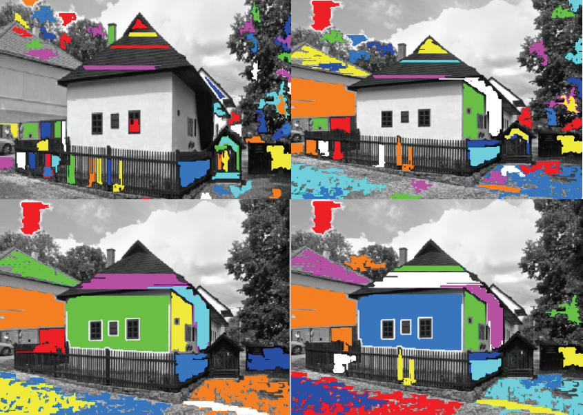
    

Example

Original image
Edge image
Highlighted image
Hue factor
Detected sky
Posted on

Recognition of car plate

Recognition of the car and finding its plate is popular theme for school projects and there are also many commercial systems. This project shows how you can recognize cars and its plate from video record or live stream. After a little modification it can by used to improve some parking systems. Idea of this algorithm is absolute different between frames and lot of testing.

Functions used: medianBlur, cvtColor, adaptiveThreshold, dilate, findContours

Input

The process

  1. Customizing the size of video footage
  2. Convert image to gray scale and blur it
    medianBlur(mainPicture,temp1,15);
    cvtColor(temp1,temp1, CV_BGR2GRAY);
    
  3. Start making absolute different between every 4 frames
  4. Threshold picture with number of thresh is 20 and number of maxval is 255
    adaptiveThreshold(temp1, temp1, 255, ADAPTIVE_THRESH_GAUSSIAN_C, THRESH_BINARY_INV, 35, 5);
    
  5. Make 25 iterations of dilation
    dilate(output,output,Mat(),Point(-1,-1), 25,0);
    
  6. Find contures from actual picture and take the area of the biggest conture
    findContours( picture.clone(), contours, CV_RETR_LIST, CV_CHAIN_APPROX_SIMPLE);
    
  7. Now you have color picture of whole car and the next step is to find a car light. Plate is somewhere between car lights.
  8. Another conversion to gray scale, erosion, dilation and blur
  9. Now threshold picture with thresh number 220 and maxval number 255
  10. Split picture to right part and left part
  11. Find biggest conture for both sides of the picture
  12. Make rectangle with both contures in it and slightly wides

Sample

Step 2 – Grey scale and blurring
Step 5 – Dilation
Step 6 – Finding the biggest conture
Step 8 – Thresholding

Result

Recognition of the car plate

// oznacenie praveho a laveho svetla
polylines(tempCar, areaR, true,Scalar(0,255,0), 3, CV_AA);
polylines(tempCar, areaL, true,Scalar(255,0,0), 3, CV_AA);

//najdenie miesta kde by sa mala nachadzat SPZ
if(!areaL.empty() && !areaR.empty() ){
//if( contourArea(Mat(areaL)) - contourArea(Mat(areaR)) < 100  ) {
      for(int i = 0; i < areaL.size(); i++){
           areaR.push_back(areaL[i]);
      }
      Rect rectR = boundingRect(areaR);
      if(rectR.width < 285 && rectR.width > 155 && rectR.height > 4 && rectR.height < 85){
            rectR.height = rectR.height + 30;
            rectangle(tempCar, rectR, CV_RGB(255,0,0));
      }
}
Posted on

Presenting historical changes of building

The goal of this project is to implement algorithm that extract similar points or whole regions from two different images of the same building using OpenCV library and especially MSER algorithm (Maximally stable extremal regions). Images of building are taken in different time and have different hue, saturation, light and other conditions.

Based on the extracted regions, algorithm finds the same centers of key regions and merged images by these points to create a complete images of building with the presentation of its historical changes.

Functions used: MSER, fitEllipse, adaptiveThreshold, Canny, findContours

Input

The process

  1. Preprocessing
  2. MSER regions detection
    MSER mser(int _delta, int _min_area, int _max_area, float _max_variation, float _min_diversity, int _max_evolution, double _area_threshold, double _min_margin, int _edge_blur_size);
    

    MSER algorithm with different parameters
  3. Fitting detected regions by ellipse
    const vector<Point>& r;
    RotatedRect box = fitEllipse(r);
    
  4. Finding similar regions
  5. Merging images based on found regions

Practical Application

Interactive presentation of the historical buildings and visualising their changes in time.

Posted on

Bag of Words Classifier

In computer vision and object recognition, we have three main areas – object classification, detection and segmentation. Classification task deals only with assigning an image to a class (for example bicycle, dog, cactus, etc…), detection task moreover deals with detecting the position of the object in an image and segmentation task deals with finding the detailed contours of the object. Bag of words is a method which belongs to classification problem.

Algorithm steps

  1. Find key points in images using Harris detector.
    Ptr<DescriptorMatcher> matcher = DescriptorMatcher::create("FlannBased");
    Ptr<DescriptorExtractor> extractor = DescriptorExtractor::create("SIFT");
    Ptr<FeatureDetector> detector = FeatureDetector::create("HARRIS");
    
  2. Extract SIFT local feature vectors from the set of images.
    // Extract SIFT local feature vectors from set of images
    extractTrainingVocabulary("data/train", extractor, detector, bowTrainer);
    
  3. Put all the local feature vectors into a single set.
    vector<Mat> descriptors = bowTrainer.getDescriptors();
    
  4. Apply a k-means clustering algorithm over the set of local feature vectors in order to find centroid coordinates. This set of centroids will be the vocabulary.
    cout << "Clustering " << count << " features" << endl;
    Mat dictionary = bowTrainer.cluster();
    
    cout << "dictionary.rows == " << dictionary.rows << ", dictionary.cols == " << dictionary.cols << endl;
    
  5. Compute the histogram that counts how many times each centroid occurred in each image. To compute the histogram find the nearest centroid for each local feature vector.

Histogram

We trained our model on 240 different images from 3 different classes – bonsai, Buddha and porcupine. We then computed the following histogram which counts how many times each centroid occurred in each image. To find the values of the histogram we had to compare the distances of each local feature vector with each centroid and centroid with least difference to local feature vector has incremented in histogram. We used 1000 cluster centers.

Posted on

Concrete Analysis

Description

In this work, we have detected a metallic wires on slide concrete. Metal parts are distributed randomly. It may happen that the positions of two adjacent wires or also cutting the wires along the length. Some wires are due to bad picture almost invisible. The images we applied filters from the library OpeCV and we have created an application that can recognize about 90% of the wires.

Input

Processing

  1. Create marker of image
    cv::erode(_grayScale, marker,
        cv::getStructuringElement(cv::MORPH_ELLIPSE,
        cv::Size(20, 20), cv::Point(-1,-1)), cv::Point(-1,-1), 2,
        cv::borderInterpolate(1, 15, cv::BORDER_ISOLATED));
    ImReconstruct(&amp;(IplImage)marker, &amp;(IplImage)_grayScale);
    

  2. Substraction grayscale image and marker image
    grayScale = _grayScale - marker;
    

  3. Use some morphological operation and get contours
    // Closing, erode, treshold
    cv::findContours(grayScale.clone(), contours, CV_RETR_TREE, CV_CHAIN_APPROX_SIMPLE, cv::Point(0,0) );
    
  4. Detailed analysis of the use of wires, in specific cases

  5. Final output

Posted on

Dominant Orientation Templates

Description

Dominant orientation templates (DOT) is a method for real-time object detection, which works well for detection of untextured objects and is related to method Histogram of oriented gradients. DOT is neither based on statistical learning of object’s shapes nor on feature point detection, but it uses real-time Template Matching recognition with locally most dominant orientations from HoG.

OpenCV function used

cvCaptureFromAVI, cvtColor

The process

  1. Computation of gradients for each pixel in template and input image
    1. Provided by convolution kernel
    2. For each pixel
    3. Gradient is defined by magnitude and direction
    4. 0-180° instead of 0-360° range
    5. Directions can be discretized from 0-180° into bins (e.g. 9 bins by 20° )
    for (int r=0;r<=area.rows-region_size;r+=region_size)
    {
        for (int s=0;s<=area.cols-region_size;s+=region_size)
        {
            int mag=gradienty_template.gradient[i][j].magnitude;
            n0=histogram_group(gradienty_template.gradient[i][j].direction);
            if (mag>min_magnitude)
                template_hist.hist_matrix[hx][hy].bins[n0]+=mag;
        }
    }
    
  2. Dividing pixels into regions

    for (int r=0;r<=area.rows-region_size;r+=region_size)
        // moving in the picture with step size of 7 or 9
    
  3. Computing most dominant gradient orientations for each region

    if (template_hist.hist_matrix[i][j].bins[k]>max) //now only the most dominant
    {
        if  (template_hist.hist_matrix[i][j].bins[k]>min_magnitude)
        {
            max=template_hist.hist_matrix[i][j].bins[k];
            max_index=k;
        }
    }
    
  4. Template matching and comparing of most dominant orientations.
  5. Evaluating comparison.

Posted on

Eye Blinking Detection

Description

The main purpose of this work is to detect eyes and recognize when are open and when close. To execute this purpose we must use video camera or video file with person face.

Eye Detection

To detect eye blinking we need to recognize face and eyes on image. For this intention we use Viola Jones algorithm which detect this features and bounded it with rectangles.

Because this algorithm is performance consuming, we use tracking which is more faster. We use Good Features to Track algorithm which return set of points suitable to track, and then with Lucas-Kanade tracker algorithm we track it on every frame.

// track points
calcOpticalFlowPyrLK(prevGray, gray, features, cornersB, status, error, Size(31, 31), 1000);

if(!calculateIntegralHOG(gray(rectangleFace)))
    text = "CLOSED";

There is problem with points which is not precisely targeted to next frame, so we remove them from set of tracking points. When number of points is not enough to track, we repeat eye detection method again.

Eye Blinking Detection

To detect if eyes are open or close we use HOG descriptor which return array of floats representing lines orientation. Because HOG descriptor is usable only on images with specific resolution, we use sliding window with this resolution which covers our image.

cv::gpu::HOGDescriptor gpu_hog(win_size, Size(16, 16), Size(8, 8), Size(8, 8), 9, 0.8, 0.00015, true);

// calculate HOG for every window
GpuMat gpuMat;
gpuMat.upload(cropped);
GpuMat descriptors;
gpu_hog.getDescriptors(gpuMat, win_size, descriptors);
Mat descriptorMat = Mat(descriptors);

In next step we take array of floats returned from HOG descriptor and transform it to histogram. We notice, that when eye is closed the local maximum of this histogram is much lower than local maximum of opened eye, so we define the value which separate opened and closed eye.

Because we use sliding window, we average all this local maxims and based on returned value, we decide if specified area contains open or close eyes.

Posted on

Google Street View Video

Description

The goal of this project is to create a program that will be able to stitch a sequence of images fromgoogle street-view and make movie from it. The idea came to my mind, when I needed to check thecrossroads and traffic signals along the route I’ve never driven before. The method was tointerpolatefew more images between two consecutive views to simulate moving car. To do that Ihad to do following steps:

Process

  1. Remove UI elements from images
  2. Find homography between following images
  3. Interpolate homography between them
  4. Put images into movie

Removing UI elements from images

Removing UI elements is important because in later steps I will need to find similar areas and those elements can spoil the match-up. First I cycled through all images and gained areas with same color in black. The resulting image was accumulated from all the differences. Black areas represent pixels that were same in all images. To improve the mask I inverted the image did some thresholding, Gaussian blur and again thresholding. Result was mask used for inpaint method to fill in those regions without UI elements with color.

Example of process

Finding homography

Homography found between two images was found using SURF detector. I improved the detection by using mask of similar areas as in previous step. I did it because many key-points were detected on sky or far objects and results were generally worse. Last step was to interpolate from one image to another using homography. In my program I used 25 steps between two pictures. Those pictures were stacked into movie and saved.

Mat homo = findMatch(pic1, pic2);
bj_corners[0] = cvPoint(0,0)
////-- Get the corners from the image_1 ( the object to be "detected" )
vector<Point2f> obj_corners(4);
obj_corners[0] = cvPoint(0,0);
obj_corners[1] = cvPoint( pic2.cols, 0 );
obj_corners[2] = cvPoint( pic2.cols, pic2.rows );
obj_corners[3] = cvPoint( 0, pic2.rows );


vector<Point2f> corners(4);
vector<Point2f> inter_corners(4);
perspectiveTransform( obj_corners, corners, homo);
...
...
for(int i=0; i<4; i++) {
 inter_corners[i].x = corners[i].x - distance[i].x*j;
 inter_corners[i].y = corners[i].y - distance[i].y*j;
}
Mat interHomo = findHomography( corners, inter_corners, 0 );
Mat transformed;
warpPerspective(pic1, transformed, interHomo, Size(600,350));
result[j] = transformed;
Posted on

Face Verification

Description

Project deals with face recognition and verification of person. It processes set of images on wich it trains eigenface and fisher face recognizer. Source of images can be csv file or web camera. When images are loaded program tries to recognize faces from set of test images and from web camera. Confidance is computed from detection which is used to verify owner of the face.

OpenCV function used

detectMultiScale, equalizeHist, createEigenFaceRecognizer, createFisherFaceRecognizer

The process

  1. Selecting and sorting images according to people (optional)
  2. Wrintting appropriate csv file (optional)
  3. Histogram equalization
  4. Face detection
  5. Add face and its label to vectors
  6. Train recognizer on saved images
  7. Predict from csv or camera

Detection phases

  1. Preprocessing (improve contrast in order to the intensity range- better illumination handling)
  2. Filtration and keypoints detection (nose holes, lips ends), available detectors: SIFT, SURF, FAST
  3. Used 2 recognizers
    1. Eigenfaces recognizer
    2. Fisher face recognizer

Sample

  1. Input image
  2. Haar face detection
  3. Conversion to grayscale
  4. Histogram equalization
  5. Recognizer training
    => RECOGNIZER
  6. Face verification
bool calculateMetrics( cv::Mat &face, bool drawToFrame )
{
std::vector<cv::Rect> eyes;
std::vector<cv::Rect> nose;
std::vector<cv::Rect> mouth;

cv::Mat canvas = faceFrameColor.clone();

// Detect eyes
eyes_cascade.detectMultiScale ( face, eyes,  1.1, 2, 0|CV_HAAR_SCALE_IMAGE, cv::Size(30, 30) );
if ( eyes.size() >; 1 && abs(eyes[0].y - eyes[1].y) < faceSize/5 && abs(eyes[0].x - eyes[1].x) > eyes[0].width)
{
    if (eyes[0].x < eyes[1].x) {
        leftEyeRect = eyes[0];
        rightEyeRect = eyes[1];
    } else {
        leftEyeRect = eyes[1];
        rightEyeRect = eyes[0];
    }
    if ( drawToFrame ) {
       rectangle(canvas, eyes[0], cv::Scalar(128,255,255), 2 );
       rectangle(canvas, eyes[1], cv::Scalar(128,255,255), 2 );
    }
    // Detect nose
    nose_cascade.detectMultiScale ( face, nose,  1.1, 2, 0|CV_HAAR_SCALE_IMAGE, cv::Size(30, 30) );
    if ( nose.size() > 0 && nose[0].y > eyes[0].y && ARE_ORDERED( eyes[0].x, nose[0].x, eyes[1].x ) )
    {
       noseRect = nose[0];
       if ( drawToFrame ) rectangle(canvas, nose[0], cv::Scalar(255,128,128), 2, 8 );

       // Detect mouth
       mouth_cascade.detectMultiScale( face, mouth, 1.1, 2, 0|CV_HAAR_SCALE_IMAGE, cv::Size(30, 30) );
       if ( mouth.size() > 0 && mouth[0].y + mouth[0].height > nose[0].y + nose[0].height && ARE_ORDERED( eyes[0].x, mouth[0].x, eyes[1].x ))
       {
           mouthRect = mouth[0];
           if ( drawToFrame ) {
               rectangle(canvas, mouth[0], cv::Scalar(64,255,64), 2, 4 );
               cv::imshow( "Face parts", canvas );
               cv::waitKey(33);
           }
       return true;
       }
    }
}
    return false;
}
Posted on

Dices Result Recognition

Description

The goal of this project is to implement algorithm that finds dots on dices. Motivation was idea / question how to create home-made random number generator? We can throw dices and our application will be able to recognize summary value on dices.

This program uses fitEllipse() function to find dots on dices. The basics steps are as follows:

Process

  1. Open video stream
    CvCapture* capture = cvCaptureFromCAM( CV_CAP_ANY );
    
  2. For the whole stream we create single frame
    IplImage* frame = cvQueryFrame( capture );
    
  3. Invert color
  4. Use adaptive threshold
    adaptiveThreshold(image, bimage, 255, ADAPTIVE_THRESH_GAUSSIAN_C, CV_THRESH_BINARY, 15, -10);
    
  5. We can use morphological operations (dilatation, erosion) to expand/minimize contours
  6. To find circles we use following:
    Mat pointsf;
    Mat(contours[i]).convertTo(pointsf, CV_32F);
    RotatedRect box = fitEllipse(pointsf);
    
  7. If difference between box.size.width and box.size.height is lower than treshold, we consider ellipse as circle.
  8. At this point we have a lot of “circles”. An experimenting helped us to determine, which circle in the picture is real point on dice. Based on size of real dices points we can isolate only real dices points.

Example of process

Original grayscale image
Inverted colors
Adaptive threshold – 255 (invert)
Histogram of points size
Lots of custom settings
RESULT!

Using custom settings we are able to improve results in specific situations.

findContours(bimage, contours, CV_RETR_LIST, CV_CHAIN_APPROX_NONE);

Vector<pair<RotatedRect*, int>> vec, finalVec;
Mat cimage = Mat::zeros(bimage.size(), CV_8UC3);
int i;
int w, h, wAhThr, angleThr, centerThr;
int  hwDifferenceThreshold, histThreshold;						
centerThr = settCenterThr;
wAhThr = settwAhThr;
hwDifferenceThreshold = settHWdifferenceThr;
histThreshold = settHistogramThr;

for(i = 0; i < contours.size(); i++)
{
	size_t count = contours[i].size();
	if( count > 50 || count  < 6)
	      continue;

	Mat pointsf;
	Mat(contours[i]).convertTo(pointsf, CV_32F);
	RotatedRect box = fitEllipse(pointsf);

	w = box.size.width;
	h = box.size.height;

	int hwDifference = abs(h - w);
	if (hwDifference > hwDifferenceThreshold)
	      continue;

	if (w < wAhThr || h < wAhThr)
	      continue;

	vec.push_back(pair<RotatedRect*, int>(new RotatedRect(box), i));
}

int asdf = vec.size();
Vector<pair<RotatedRect* ,int>>::iterator it ,iend, it2;
int MAXHIST = 200;
int* histVals = new int[MAXHIST];
for (int i = 0; i < MAXHIST; i++)
	histVals[i] = 0;

int histIter = 0;
RotatedRect * box;
RotatedRect * box2;
int maxWidth = 0;
int distanceOfCenters;
for (it = vec.begin(), iend = vec.end(); it != iend; it++)
{
	box = (it->first);
	for (it2 = it + 1; it2 != iend; it2++)
	{
		box2 = (it2->first);
		distanceOfCenters = (int)std::sqrt((box->center.x - box2->center.x) * (box->center.x - box2->center.x) + (box->center.y - box2->center.y)  * (box->center.y - box2->center.y));
		if (distanceOfCenters < centerThr)
		{
			if (box->size.width > box2->size.width)
				it2->second = -1;
			else
				it->second = -1;
			break;
		}

	}
}
Posted on

Moving Vehicle Detection

The goal of this project is to implement algorithm that segments foreground using OpenCV library. We assume that background is static, objects in foreground are moving and video is taken from static camera. We detect moving  vehicles (foreground) with 2 methods.

Background detection

First method is computing an average image from video frames.

  1. Each frame is added into accumulator with a certain small weight (0.05 and smaller)
    1. accumulateWeighted(frame, background, alpha);
    2. at this point we have in Mat background actual backgorund image
  2. To detect foreground we have to compute difference between current frame and current accumulated background image
    1. absdiff(frame, background, diff);
    2. in Mat diff is color image, we need to transform it into grayscale image
  3. To detect relevant changes (more than given threshold) we use simple
    1. thresholdthreshold(diff, foregroundMask, 20, 255, CV_THRESH_BINARY);
    2. in Mat foregroundMask is foreground mask
  4. We can use morphological operations (dilatation, erosion) to expand foreground region

Each steps (1-4) are illustrated in next figures

Frames history

Second method is compare current frame with older frame. It is enough if the stack is 5-20 elements large- it depends on the speed of vehicles.

  1. Add current frame into stack (if stack is full, first element is erased and the rest is shifted)
    1. framesHistory.add(frame);
  2. Compute difference between current frame and first element in the stack
    1. first = framesHistory.first();
    2. absdiff(frame, first, diff);
  3. To detect relevant changes (more than given threshold) we use simple threshold
    1. threshold(diff, foregroundMask, 20, 255, CV_THRESH_BINARY);
    2. in Mat foregroundMask is foreground mask
  4. We can use morphological operations (dilatation, erosion) to expand foreground region

Each steps (1-4) are illustrated in next figures. LocalBackgound is the older frame (5 frames old)

Combination of methods

These 2 methods are combined to create more accurate output. In the next picture we can see that first way (computing average image) creates “tails” behind vehicles. Comparing with older frame doesn’t create „tails“.

We use simple sum of binary masks

Mat sumMask = mask1 & mask2

How to create more precise segmentation, future work

To create more precise vehicle segmentation we have to use another methods. Shadows of cars, lights of cars make these 2 methods to hard use. We can only segment region where could be a car, but for more precisely detection we have to use template matching (champfer matching), graph cut method. In this project we experimented with these other two, but these were too complex, so the time complexity was unacceptable to use in video.

Posted on

CSS – Curvature Scale Space in OpenCV

Description

The goal of this project is to implement algorithm that creates curvature scale space (CSS) image of given shape using OpenCV library. “The CSS image consists of several arch-shape contours representing the inflection points of the shape as it is smoothed. The maxima of these contours are used to represent a shape. The CSS representation is robust with respect to scale, noise and change in orientation.”[1]

CSS representations for various curve modifications [1]

Process

  1. Find contour coordinates of given shape
  2. findContours(im, contours, CV_RETR_LIST, CV_CHAIN_APPROX_NONE );
    

    Following steps are repeated with increased sigma until there are no zero-crossing points:

  3. Gaussian kernel is the base for upcoming steps:
    transpose(getGaussianKernel(width, sigma, CV_64FC1), G);
    
  4. Curve evolution can be computed by convolution of contour points with Gaussian kernel. Smoothed contour is not needed for CSS computation; it is used only to visualize the process:

    filter2D(X, Xsmooth, X.depth(), G);
    filter2D(Y, Ysmooth, Y.depth(), G);
    

    Curve evolution with increasing sigma [2]
  5. To compute 1st and 2nd derivation of contour points, Gaussian kernel derivations will be needed:
    Sobel(G, dG, G.depth(), 1, 0, 3);
    Sobel(G, ddG, G.depth(), 2, 0, 3);
    
  6. Convolution of contour points using derivatives of Gaussian kernel. According to OpenCV documentation: filter2D does actually computes correlation, not the convolution. That is, the kernel is not mirrored around the anchor point. If you need a real convolution, flip the kernel using flip() and set the new anchor to (kernel.cols – anchor.x – 1, kernel.rows – anchor.y – 1) :
    flip(dg, dg, 0);
    flip(ddg, ddg, 0);
    Point anchor(dg.cols - fwhm -1, dg.rows - 0 - 1);
    filter2D(X, dX, X.depth(), dG, anchor);
    filter2D(Y, dY, Y.depth(), dG, anchor);
    filter2D(X, ddX, X.depth(), ddG, anchor);
    filter2D(Y, ddY, Y.depth(), ddG, anchor);
    
  7. Finally, we calculate the curvature and find zero crossings:

    Curvature and inflection points of curve smoothed with sigma=16
  8. Zero-crossing points are plotted to the final CSS image. X-axis represents position of point on the curve; Y-axis represents the value of sigma:
    Final CSS image with zero-crossing points for all sigmas

Practical Applications

  • Finding similar shapes  (Used as shape descriptor in MPEG-7 standard)
  • Corner detection
Example of cornes detection

References

[1] Sadegh Abbasi, Farzin Mokhtarian, Josef Kittler: Curvature Scale Space Image in Shape Similarity Retrieval. Multimedia Syst. 7(6): 467-476 (1999)

[2] Farzin Mokhtarian, Alan K. Mackworth: A Theory of Multiscale, Curvature-Based Shape Representation for Planar Curves. IEEE Trans. Pattern Anal. Mach. Intell. 14(8): 789-805 (1992)